How accurate are numbers inferred from measurements and simulations?
“Uncertainty quantification” (or “UQ” for short) is a research area that has sprung to prominence in the last decade at the interface of applied mathematics, statistics, computational science, and many applications, usually in physical sciences and engineering, but also in biology, finance, and insurance.

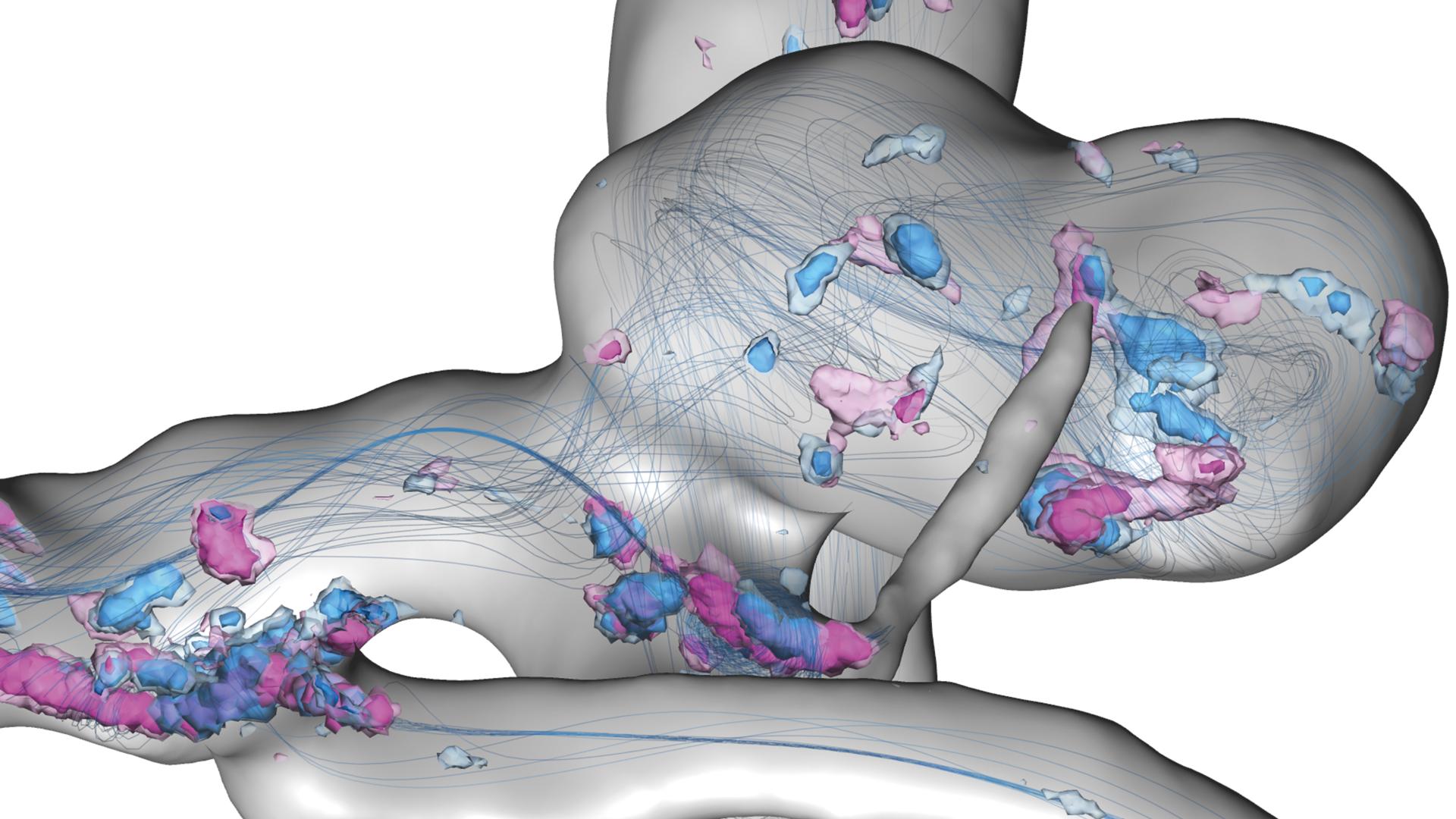
Uncertain flow features in a cerebral aneurysm within a full heart cycle: Depicted are streamlines of the simulated time-averaged blood velocity and spatial probabilities of critical points with Poincaré index > 0 and < 0 – visualized by blue and violet isosurfaces, respectively.
Uncertainty Quantification
In all these applications, there is a real and growing demand to synthesize complex real-time data sets and historical records with equally complex physically-based computational models for the underlying phenomena, in order to perform tasks as diverse as extracting information from novel imaging techniques, designing a new automobile or airplane, or predicting and mitigating the risks arising from climate change.
Simply put, UQ is the end-to-end study of the impact of all forms of error and uncertainty in the models arising in the applications. The questions considered range from fundamental, mathematical, and statistical questions to practical questions of computational accuracy and cost (FN:T. J. Sullivan. Introduction to Uncertainty Quantification. Springer, 2015.). Research into these questions takes place at ZIB in the Uncertainty Quantification group, and finds applications in other working groups such as Computational Medicine, Computational Molecular Design, and Visualization.
A general introduction to UQ and Bayesian inverse problems
 = p(Y|X) p(X) / p(Y)")
Roughly speaking, UQ divides into two major branches, forward and inverse problems. In the forward propagation of uncertainty, we have a known model F for a system of interest. We model its inputs X as a random variable and wish to understand the output random variable Y = F(X), sometimes denoted Y|X, read as “Y given X.” There is a substantial overlap between this area and sensitivity analysis, since the random variations in X probe the sensitivity of the forward model F to changes of its inputs. In the other major branch of UQ, inverse problems, F is still the forward model, but now Y denotes some observed data, and we wish to infer inputs X so that F(X) = Y; that is, we want not Y|X but X|Y. Here, there is substantial overlap with statistical inference and with imaging and data analysis. Inverse problems typically have no solutions in the literal sense, because our models F are only approximate, there is no X for which F(X) agrees exactly with the observed data Y. Therefore, it becomes necessary to relax the notion of a solution, and often also to incorporate prior or expert knowledge on what a “good” solution X might be. In recent years, the Bayesian perspective on inverse problems has received much attention, because it is powerful and flexible enough to meet these requirements, and because increased computational power makes the Bayesian approach more feasible than in decades past (FN:A. M. Stuart. Inverse problems: A Bayesian perspective, Acta Numer. 19:451559, 2010.). In the Bayesian perspective, we again regard X and Y as random variables and encode our prior expert knowledge about X into a prior probability distribution p(X), which we condition with respect to Y using Bayes’ rule
p(X|Y) = p(Y|X) p(X) / p(Y)
to produce a so-called posterior distribution for X|Y, which is the mathematical representation of all knowledge/uncertainty about X, given the observed data Y and the expert knowledge encoded in the prior p(X). However, the posterior p(X|Y) is typically a very complicated distribution on a large space (the space of unknown Xs that we are trying to infer), so there are major mathematical and computational challenges in implementing this fully Bayesian approach, and in producing appropriate simplifications for end users.
UQ in systems biology and parameter estimation
The Systems Biology group at ZIB deals with the computational and mathematical modeling of complex biological systems: metabolic networks or cell signaling networks, for example. Usually, the models consist of large systems of ordinary differential equations that describe the change of concentrations of the involved species over time. Such models involve a huge number of model parameters representing, for example, reaction rate constants, volumes, or effect concentrations. Only a few of these parameters are measurable, sometimes their approximate range of values is known, but often their order of magnitude is completely unknown. The aim is to estimate parameter values in such a way that simulation results match with given experimental data and that predictions can be made about the system’s behavior under external influences: thus, these problems fall under the general heading of inverse problems.

Fig. 2: Schematic representation of the Bayesian approach to the construction of patient-specific physiological models for the prediction of individual treatment success rates, for example.
The data, however, are prone to measurement errors and are therefore uncertain. Given a fixed set of data and a statistical model for the error, one can solve an optimization problem to compute a single set of parameter values that make the observed data the most probable given the model (FN:D. P. Moualeu-Ngangue, S. Röblitz, R. Ehrig, P. Deuflhard. Parameter Identification in a Tuberculosis Model for Cameroon. PLoS ONE 10[4]:e0120607. doi:10.1371/journal.pone.0120607, 2015.). The function to be optimized is called likelihood function. In practice, this optimization problem is often difficult to solve, because its solution is not unique. In other words, there exist several different sets of parameter values that all lead to equally good fits to the data.
Alternatively, when prior knowledge about the parameters is postulated, parameters can be treated as random variables in the framework of Bayesian statistics. This allows you to compute a joined probability distribution for the parameters, called the posterior. Performing model simulations with parameters sampled from this posterior distribution gives insight into the variability and uncertainty of the model output.
A possible application is the prediction of patient-specific treatment success rates based on a physiological model for a specific disease or health status. Given some measurement data from a large group of patients, one can construct a prior distribution that reflects the variability of parameters within the patient population (FN:I. Klebanov, A. Sikorski, C. Schütte, S. Röblitz. Prior estimation and Bayesian inference from large cohort data sets. ZIB-Report 16-09. Zuse Institute Berlin, 2016.). Using this prior and a patient-specific data set, an individual posterior can be computed. Running model simulations including the treatment with parameters sampled from the posterior then allows us to quantify the failure probability of the treatment and to analyze under which conditions a treatment fails for a specific patient.
UQ in optical metrology
Optical metrology uses the interaction of light and matter to measure quantities of interest, like geometry or material parameters. Reliable measurements are essential preconditions in nanotechnology. For example, in the semiconductor industry, optical metrology is used for process control in integrated circuit manufacturing, as well as for photomask quality control. In this context, measurements of feature sizes need to be reliable down to a sub-nanometer level. As the measurement amounts to solving an inverse problem for given experimental results, methods for both simulating light-matter interaction in complex 3-D shapes and uncertainty quantification are required.
A typical experimental setup consists of a well-defined light source, the scattering object, and a detector for the scattered light. Figure 3 shows a setup with fixed illumination wavelength and variable settings for polarization and direction of incident and detected light components. However, wavelength-dependent measurements are also typical in optical metrology. The detected spectra are used to reconstruct the scattering structure. The choice of illumination and detection conditions directly impacts the measurement sensitivity. The scatterers to be analyzed are manifold in the semiconductor industry, for example. Gratings, as well as active components like FinFETs or VNANDs, are of interest.

Fig. 3: Goniometric deep ultraviolet scatterometer of Physikalisch-Technische Bundesanstalt.
In a collaborative study of Physikalisch-Technische Bundesanstalt (PTB) and ZIB’s research group on Computational Nano Optics, the grating shown in Figure 4 (left) has been studied. Its geometric parameters, as shown in Figure 5, have been identified by a Gauß-Newton method. Reconstruction results are summarized in Table 1. The simulated spectral reflection response for the reconstructed parameters matches the experimental data very closely. Estimating the posterior covariance by local Taylor approximation reveals a satisfactory accuracy and indicates the high quality of the implemented models (FN:S. Burger, L. Zschiedrich, J. Pomplun, S. Herrmann, F. Schmidt. hp-finite element method for simulating light scattering from complex 3D structures. 9424: 94240Z, 2015.). Hence, the approach is a promising candidate for investigations of far more complex semiconductor structures, as exemplarily shown in the center and bottom parts of Figure 4.
 of a prototype of a scatterometry reference standard sample, manufactured at Helmholtz-Zentrum, Berlin. Center: Simplified geometry model of a 3-D NAND structure for memory chips. Bottom: Simplified geometry model of a FinFET semiconductor component.")
Fig. 4: Top: Microscopic image (SEM) of a prototype of a scatterometry reference standard sample, manufactured at Helmholtz-Zentrum, Berlin. Center: Simplified geometry model of a 3-D NAND structure for memory chips. Bottom: Simplified geometry model of a FinFET semiconductor component.

Fig. 5: Geometry model for the sample shown in Figure 2.

Molecular design
THE Challenge FOR Computational Molecular Design
Molecular systems have metastable states with low transition probabilities between these states. For the optimal design of interacting molecules (drugs, analytes, sensors) it is often very important to adjust some of these transition probabilities by redesigning parts of the molecular system, in order to increase affinity or specificity, for example. The Computational Molecular Design group predicts the essential transition probabilities of molecular systems on the basis of molecular dynamics (MD) simulations. To save on computational costs, one aims at extracting the essential transition probabilities from as few as possible short MD simulations. The trajectories that result from each of these simulations can be considered as observed data that are used to infer the desired transition probabilities.
Uncertainty of transition probabilities
The challenge for the Computational Molecular Design group is to compute the long-term behavior of molecular systems on the basis of only a few short-time molecular simulations. Molecular systems exhibit a multiscale
dynamical behavior: they undergo rare transitions between metastable states, for example. If the statistical analysis of these transitions is based on a few short-time simulations (the observed data Y) only, then the correct transition probabilities (the inferred unknowns X) are uncertain. In this case the posterior distribution for X|Y is a distribution on transition matrix space that reflects the uncertainty about the transition matrix X, given the observed simulation data Y and the expert knowledge encoded in the prior p(X). Applying appropriate UQ algorithms leads to an ensemble of transition matrices. This ensemble of transition matrices allows us to compute the uncertainty in the quantities extracted from the transition matrices, the dominant timescales of the system, for example. It was recently demonstrated how to utilize the insight into these uncertainties for understanding the physical/chemical meaning of the indeterminacy of metastable states (FN:M. Weber, K. Fackeldey: Computing the Minimal Rebinding Effect Included in a Given Kinetics. Multiscale Model. Simul., 12[1]:318-334, 2014.) which led to new design principles for synthetic chemistry (FN:C. Fasting, C.A. Schalley, M. Weber, O. Seitz, S. Hecht, B. Koksch, J. Dernedde, C. Graf, E.-W. Knapp, R. Haag. Multivalency as a Chemical Organization and Action Principle, Angew. Chem. Int. Ed. 51[42]:10472–10498, 2012.).
Incomplete simulation data
If only some and not all of the essential transition probabilities are known, then the corresponding transition matrix is incomplete, or some entries are missing. We have constructed matrix completion algorithms for estimating these entries on the basis of the given simulation data without performing further simulations, which saves a lot of computational effort. In order to estimate the unknown entries, different assumptions are useful. One can consider a low-rank transition matrix, or assume the matrix to be doubly-stochastic and comprise only some major transition paths, or that it is a similarity matrix of a small number of clustered objects.
Changing the molecular structure
Another important question is how to reduce computational costs when simulating various molecular systems which only differ in some part of the molecular system that is small (Figure 6) compared to the size of the entire system. We investigated methods that allow for the prediction of transition matrices for a changed molecular system on the basis of the simulated original system (FN:Ch. Schütte, A. Nielsen, M. Weber. Markov State Models and Molecular Alchemy. Molecular Physics, 113[1]:69-78, 2015.),(FN:A. Nielsen. Computation Schemes for Transfer Operators. Doctoral dissertation, Freie Universität Berlin, 2015.). The mathematical background is based on the theory of path integrals or reweighting in path space, which plays a major role in many of our present and future projects.

Fig. 6: Often many simulations are performed with very similar molecular systems. Sometimes only one side group of a binding molecule varies, in this case in the violet region.
UQ in computer vision and geometry reconstruction
Computer Vision
Computer vision extracts numerical or symbolic information from image data, using methods for acquiring, processing, analyzing, and understanding images. If decisions are based on such information, it is important to know how reliable it is. Thus, UQ becomes necessary for processing pipelines in computer vision.
This is illustrated by the following three examples: 1) An orthopedic surgeon has to decide, based on a computed tomography (CT) scan of a patient, whether a bone is solid enough to permit fixation of a screw that holds a certain maximum load. Such a decision requires extraction of the bone’s thickness and material density – including error bounds – from the CT scan. 2) In pathology, many conclusions are drawn, based on frequencies of cell types in biopsies. Reliable diagnoses require knowledge not just of cell counts in microscopic images, but also of the uncertainties related to the identification and classification of cells. 3) In self-driving cars, potentially far-reaching decisions have to be taken based on information from video images; examples are the route and speed of the car, considering estimated trajectories of vehicles and pedestrians, for example. The uncertainty of such image-based information needs to be estimated to be taken into account.
Obviously, a wealth of research topics arises. At ZIB, research has started concerning UQ in image segmentation. In a first approach, images are considered as random fields, and spatial probabilities for membership functions are computed. This works for basic segmentation techniques that utilize only local information, like thresholding, for example. Consideration of non-local information renders UQ into a much more difficult problem. A fundamental problem is to capture the modeling uncertainty in image segmentation.

Fig. 7: Reconstruction of pelvic bone and hip joints on the basis of few X-ray projections.
Geometry Reconstruction
The 3-D shape of human anatomy, as needed in particular for surgery and therapy planning tasks, is usually extracted from 3-D image stacks provided by CT scans. Dose reduction requires a limit on the number of X-ray projections entering the CT to very few, but these do not contain enough information to reconstruct 3-D image stacks. The anatomy, however, can be described by statistical shape models in terms of a small number of parameters. Using such shape models as priors renders the Bayesian inverse problem well-posed and allows an efficient computation of maximum posterior estimates (FN:M. Ehlke, T. Frenzel, H. Ramm, M. A. Shandiz, C. Anglin, S. Zachow. Towards Robust Measurement Of Pelvic Parameters From AP Radiographs Using Articulated 3D Models. Computer Assisted Radiology and Surgery [CARS], 2015.). The research groups on Therapy Planning, Computational Medicine, and Visual Data Analysis in Science and Engineering investigate the properties of the posterior density and the design of X-ray acquisition to minimize the uncertainty.
Due to the nonlinear impact of shape changes on the projection images, the posterior density is a mixture of Gaussian and Laplacian distributions. This makes UQ by local Gaussian approximation unreliable and requires the use of sampling techniques or a more accurate modeling of the impact of nonlinearities.
Uncertainty visualization
In many applications of information processing, humans are (still) involved; examples are explorative data analysis where humans try to gain understanding or making decisions based on computed information. In such cases, information must be conveyed to humans, ideally by visualization. If the information is subject to uncertainty, this should also be communicated visually.
Research in the group Visual Data Analysis in Science and Engineering at ZIB focuses on the visualization of uncertainties in spatial and spatiotemporal data, particularly on cases where certain “features” in the data are of interest. Examples of such features are level sets, critical points, and ridges in scalar fields, or critical points in vector fields. For uncertain data that can be represented as random fields, an approach has been developed to compute and depict the resulting spatial or spatiotemporal uncertainties of such features (FN:K. Pöthkow. Modeling, Quantification and Visualization of Probabilistic Features in Fields with Uncertainties. Doctoral dissertation, Freie Universität Berlin, 2015),(FN:K. Pöthkow, H.-C. Hege [2013]. Nonparametric models for uncertainty visualization. Computer Graphics Forum. 32[3]:131–140.). Here, expectation values of feature indicators are computed with Monte Carlo methods; these can be interpreted as probabilities of the presence of a feature at some point in space or space-time.
In Scientific Computing, uncertainties are often captured by ensemble computations, where instead of a single computation many computations are performed, with varying parameters or even mathematical models. This approach is used in meteorology and climatology, for example. If the results of such ensemble computations can be summarized in random fields, our methods for uncertainty visualization apply directly.

Color-coded spatial probabilities of the 0°C isotherm in the earth’s atmosphere at some specific date. The white surface represents the isotherm of the ensemble average.