Inverse Problems
This example illustrates:
- Systems of PDEs
- Accessing matrix blocks for block solver
- Writing multiple outputs
- Passing a measurement field during assembly
and can be found at tutorial/inverse.
Background
This tutorial considers the source term inversion of an elliptic problem by identifying the volume source terms \(f\) which produces the temperature field \(T\). A synthetic measurement data is produced by the same numerical scheme for inversion, since this is considered an inverse crime noise is added to the measurement data. The method of Lagrange multipliers is used to enforce equality constraint of satisfying the state PDE. Since inverse problems are inherently ill-posed a Tikhonov regularization scheme is employed.
Mathematical Formulation
Given \(\Omega \subset \mathrm{R}^d, d \in\) {1,2} is an open bounded unit square domain and consider the following least-squares functional: \[ \min_ {f} J(f,T) = \frac{1}{2}\int_\Omega (T-T_m)^2 d\Omega + \frac{\alpha}{2}\int _{\Omega} |\nabla f|^2 d \Omega \]
Where \( \ T_m \ \) is the measured temperature field, the second term of the functional is the \(\ H1 \ \) Tikhonov regularization term where \(\ \alpha \) is the regularization parameter and \(\ T \ \) is the solution of the elliptic PDE
\[- \Delta T \kappa + Tq = f \quad \text{in } \Omega \]
\[ \nabla T \cdot n = 0 \quad \text{on }\Gamma_N \subset \Omega \]
\[ T =g \quad \text{on } \Gamma_D \subset \Omega \]
To enforce the state elliptic PDE as an equality constraint we introduce the Lagrange multiplier function \(\ \lambda \ \) to \(\ J \ \) yielding the Lagrange functional \(\mathcal{L} \)
\[ \mathcal{L} (T,\lambda,f) := \frac{1}{2}\int_\Omega (T-T_m)^2 d\Omega + \frac{\alpha}{2}\int _{\Omega} |\nabla f|^2 d \Omega + \int _{\Omega} \lambda (\nabla T \kappa + Tq - f) d \Omega \]
To derive the necessary optimality conditions the Lagrange multiplier theory states that at a solution of the Lagrange functional variations of it with respect to its variables must vanish
\[ \mathcal{L}_{\lambda}(T,\lambda,f)(\delta \lambda) = \nabla T \delta \nabla \lambda \kappa + T \delta \lambda q - f \delta \lambda =0 \]
\[ \mathcal{L}_{T}(T,\lambda,f)(\delta T)= (T-T_m) \delta T + \delta \nabla T \nabla \lambda + \delta T \lambda = 0 \]
\[ \mathcal{L}_{f}(T,\lambda,f)(\delta f)= \alpha \nabla f \delta \nabla f - \delta f \lambda= 0 \]
The above system of equations represent the weak form of the adjoint, state and control equations respectively. The strong form of the adjoint and control equations respectively is
\[ T + \Delta \lambda + \lambda = T_m \quad \text{in } \Omega \]
\[ \nabla \cdot n = 0 \quad \text{on } \Gamma \]
\[ \alpha \Delta f - \lambda = 0 \quad \text{in } \Omega \]
\[ \nabla \cdot f = 0 \quad \text{on } \Gamma \]
It is helpful for later on in the implementation to formulate the strong form as
\[ \begin{bmatrix} I&(\Delta+I)&0 \\ (\Delta \kappa+I q)&0&-I \\ 0&-I&\alpha \Delta \end{bmatrix} \begin{bmatrix} T \\ \lambda \\ f \end{bmatrix} = \begin{bmatrix} T_{m} \\ 0 \\ 0 \end{bmatrix} \]
Discretization
By employing a Galerkin discretization to the system of Lagrange optimality conditions, the discretized system of equations will be
\[ \begin{bmatrix} A_{T}&K_{\lambda} +A_{\lambda}&0 \\ (K_{T}+A_{T})&0&-A_{f} \\ 0&-A_{\lambda}&\alpha K_{f} \end{bmatrix} \begin{bmatrix} T \\ \lambda \\ f \end{bmatrix} = \begin{bmatrix} T_m v \\ 0 \\ 0 \end{bmatrix} \]
Here \(A , K \) are the mass and stiffness matrix. Since \(T,\lambda \text{ and } f \) can be discretized with different anzats functions and discretization order the resulting mass and stiffness matrix can be different for each variable hence the subscripts.
Source code documentation
In this problem the code can be divided into 2 parts Measurement generation and Source inversion with 3 files of interest (ht.hh inverse.hh inverse.cpp ).
I. Measurement generation
To generate the measurement temperature field we first solve the state equation for T:
\[- \Delta T \kappa + Tq = f \quad \text{in } \Omega \]
With pure zero Dirichlet boundary condition over the boundaries:
\[ T =0 \quad \text{on } \Gamma_D \subset \Omega \]
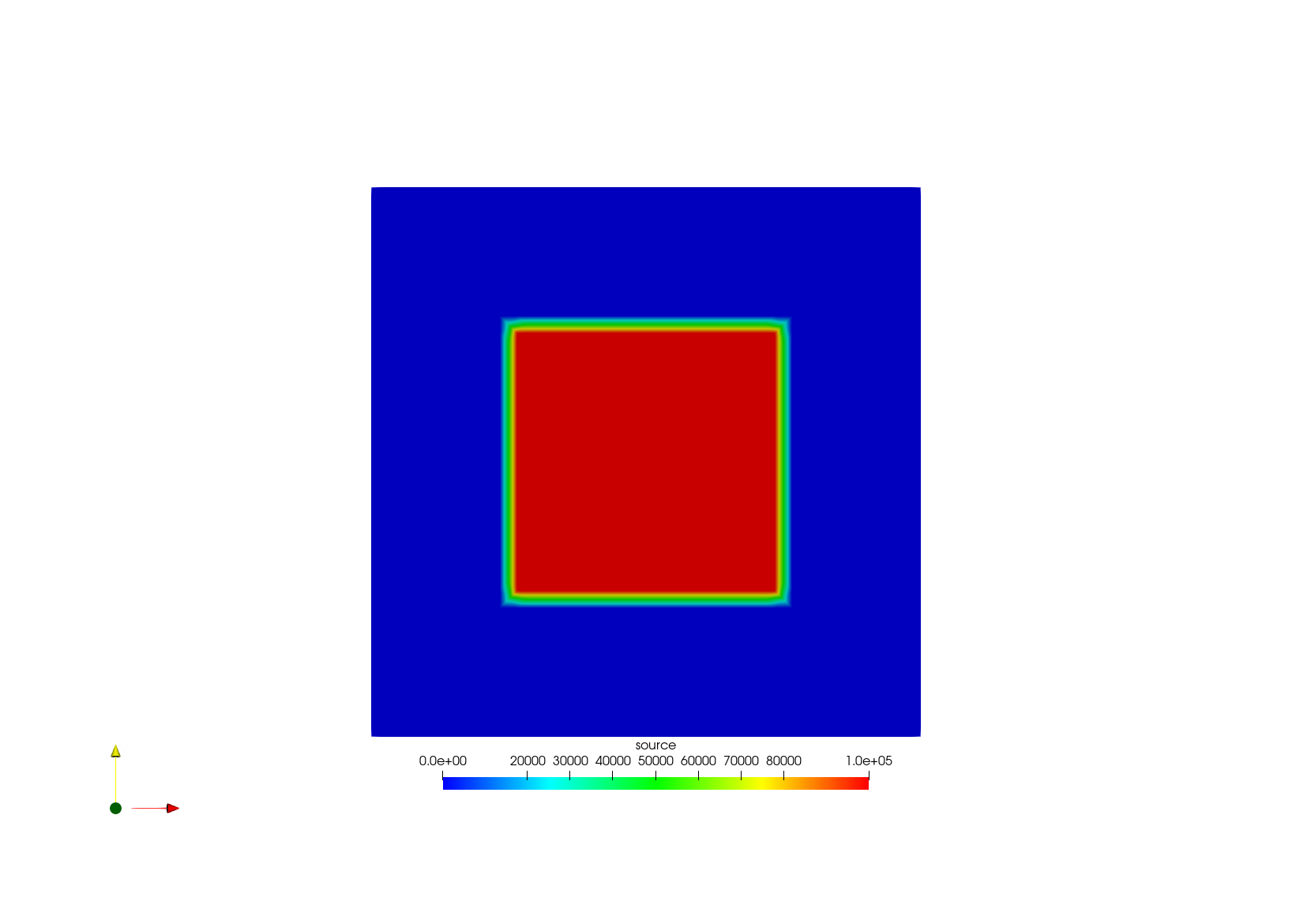
Given a distributed source term f = 10^5 over the interval:
\[ f(x,y) = \begin{cases} 10^5, & 0.25<x< 0.75 \; \wedge \; 0.25<y<0.75 \\ 0, & \text{otherwise} \end{cases} \]
Files of interest ( First block of inverse.cpp and ht.hh)
Include header files :
#include <iostream>
#include <string>
#include <random>

#include <boost/timer/timer.hpp>

#include "dune/grid/config.h"
#include "dune/grid/uggrid.hh"

#include "fem/assemble.hh"
#include "fem/norms.hh"
#include "fem/lagrangespace.hh"
#include "linalg/direct.hh"
#include "utilities/enums.hh"
#include "utilities/gridGeneration.hh" //  createUnitSquare
#include "io/vtk.hh"
#include "utilities/kaskopt.hh"

#include "ht.hh"
#include "inverse.hh"

inverse.cpp
Command line input parameters : Here we can define default parameters for the problem which can be changed from the command line when running the executable .e.g (./inverse - -refinements 4) will refine the mesh 4 times instead of the default value 5. This is useful since the program needs to be compiled once.
  std::unique_ptr<boost::property_tree::ptree> pt = getKaskadeOptions(argc, argv, verbosityOpt, dump);

  int  refinements = getParameter(pt, "refinements", 5), // Number of times the mesh is refined
       order       = getParameter(pt, "order", 1); // Discretization order

  double   kappa   = getParameter(pt, "kappa", 1.0), //The diffusion constant
           q       = getParameter(pt, "q", 1.0), //The mass coefficient
	       alpha   = getParameter(pt,"alpha",1e-6), //The regularization parameter
	       noise   = getParameter(pt,"noise",1); //Standard deviation of the added noise
inverse.cpp
Grid creation and Space definition is similar to section Hello world, with the exception of adding a Discontinuous Lagrange space for storing the source term and passing the measurement term to the inverse problem formulation in the next section.
Spaces now contain a ContinuousLagrangeMapper type H1 Space and a DiscontinuousLagrangeMapper type L2 Space, with a corresponding Space index of <0> and <1>.
  constexpr int dim=2;
  using Grid = Dune::UGGrid<dim>;
  using LeafView = Grid::LeafGridView;
  using H1Space  = FEFunctionSpace<ContinuousLagrangeMapper<double,LeafView> >;

  using L2Space  = FEFunctionSpace<DiscontinuousLagrangeMapper<double,LeafView>>; // New Space definition
  using Spaces   = boost::fusion::vector<H1Space const*, L2Space const*>;         // Combined H1 and L2 Space

  using VariableDescriptions = boost::fusion::vector<Variable<SpaceIndex<0>,Components<1>,VariableId<0> > >;
  using VariableSet = VariableSetDescription<Spaces,VariableDescriptions>;
  using Functional = HeatFunctional<double,VariableSet>;
  using Assembler = VariationalFunctionalAssembler<LinearizationAt<Functional> >;

inverse.cpp
Next we create a L2Space::Element_t<1> object this space can be used for storing values inside each cell in the meshed domain, the template parameter is for the number of values to be stored in each cell in this case it is 1.
note: The order in the created l2Space is set to 0, with this we can store a constant value in the cells.
  // construction of finite element space for the scalar solution T_m.
  H1Space h1Space(gridManager,gridManager.grid().leafGridView(),order);

  L2Space l2Space(gridManager,gridManager.grid().leafGridView(),0);

  Spaces spaces(&h1Space,&l2Space);

  //construction of L2 space with 1 component for storage
  L2Space::Element_t<1> measurementSpace(l2Space);
  L2Space::Element_t<1> sourceSpace(l2Space);

inverse.cpp
Defining the necessary source term, Domain cache and Boundary cache is similar to Timestepping, but in this problem we have an extra mass term in the DomainCache. All of which are defined in the header file ht.hh
Here using the evaluateAt member function we can define the source term f
 void evaluateAt(LocalPosition<Grid> const& x, Evaluators const& evaluators)
    {
      u  = data.template value<0>(evaluators);
      du = data.template derivative<0>(evaluators)[0];

      xglob = cell.geometry().global(x);

      if (xglob[0] >0.25 && xglob[0]<0.75 && xglob[1] >0.25 && xglob[1]<0.75 ){
       f=1e5;
      }
      else f=0.0;
    }

ht.hh
The mathematical form of the member functions d0 , d1 and d2 in theDomainCache
\[ \text{d0: } F(T) = \frac{1}{2}\kappa \nabla T^T \nabla T +qTT - fT. \] \[ \begin{aligned} &\text{d1: } F’(T)[v] = \kappa \nabla T \cdot \nabla v+ qTv - fv \\ &\text{d2: } F’’(T)[v,w] = \kappa \nabla v \cdot \nabla w + qwv \end{aligned} \]
    Scalar d0() const
    {
      return (F.kappa*du*du + F.q*u*u)/2 - f*u;
    }

    template<int row, int dim>
    Dune::FieldVector<Scalar, TestVars::template Components<row>::m>
    d1 (VariationalArg<Scalar,dim> const& arg) const
    {
      return F.kappa*du*arg.derivative[0] + F.q*u*arg.value - f*arg.value;
    }

    template<int row, int col, int dim>
    Dune::FieldMatrix<Scalar, TestVars::template Components<row>::m,
                      AnsatzVars::template Components<col>::m>
    d2 (VariationalArg<Scalar,dim> const &argT,
        VariationalArg<Scalar,dim> const &argA) const
    {
      return F.kappa*argT.derivative[0]*argA.derivative[0] + F.q*argT.value*argA.value;
    }
ht.hh
After solving the state equation using the directInverseOperator for the scalar variable \(T\) now we have the desired measurement field \(T_m\). Next we will add noise to \(T_m\) using the std::default_random_engine to generate a random number and std::normal_distribution to restrict the random number to a Gaussian distribution with the mean as \(T_M\) and the standard deviation as our input parameter noise.
To perform this operation we will make use of the interpolateGlobally, it interpolates values from one function space element to another by traversing each cell in the function space using makeFunctionView and takes a weighing scheme as a template parameter. In this problem we interpolate values from the solution space \(T_m\) which is an H1 continuous Lagrange space to our measurementSpace which is a L2 discontinuous Lagrange space.
  // create a random number generator
  std::default_random_engine generator;


  interpolateGlobally<PlainAverage>(measurementSpace,makeFunctionView(h1Space, [&] (auto const& evaluator)
  {

    double measurement= component<0>(T_m).value(evaluator) ;
    std::normal_distribution<double> distribution(measurement,noise);


    return Dune::FieldVector<double,1>( distribution(generator));

  }));

inverse.cpp
Now we have the noisy measurements stored, to visualize the resulting source term we can make use again of interpolateGlobally to store its values.
  //Storing the source field for visualization

  interpolateGlobally<PlainAverage>(sourceSpace,makeFunctionView(h1Space, [&] (auto const& evaluator)
  {

    auto   x = evaluator.cell().geometry().center();
    double f=0;

   if (x[0] >0.25 && x[0]<0.75 && x[1] >0.25 && x[1]<0.75 ) f=1e5;

    return Dune::FieldVector<double,1>(f);

  }));

inverse.cpp
The resulting source distribution is visualized in the output VTU file Source.vtu
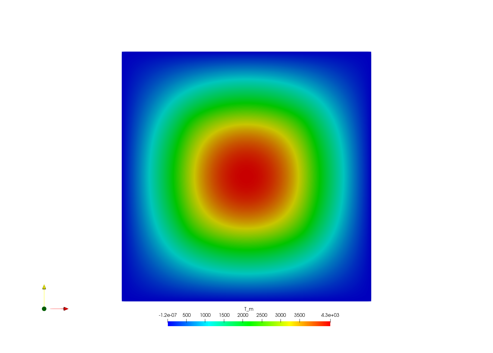
The resulting temperature field in temperature.vtu
II. Source term identification
For setting up the system of equations we first need to define 3 variables \(T, \lambda, f \) in the VariableDescriptions along with redefining the Classes depending on it VariableSet , Functional and Assembler. Here, the space index for all the variable is set to <0> this means all the variables will be discretized using the \(H1\) continuous Lagrange polynomials of the same order.
Here, one also can choose a different discretization for each variable by creating the desired space and assigning the variable to it.
Note: The capital I is for indicating the inverse problem related definitions.
  using IVariableDescriptions = boost::fusion::vector<Variable<SpaceIndex<0>,Components<1>,VariableId<0>>,
                                                      Variable<SpaceIndex<0>,Components<1>,VariableId<1>>,
                                                      Variable<SpaceIndex<0>,Components<1>,VariableId<2>>>;

  using IVariableSet        = VariableSetDescription<Spaces,IVariableDescriptions>;
  using IFunctional         = IHeatFunctional<double,IVariableSet>;
  using IAssembler          = VariationalFunctionalAssembler<LinearizationAt<IFunctional> >;


  std::string  IvarNames[3] = { "T","lambda","f" };
  IVariableSet IvariableSet(spaces,IvarNames);
  IFunctional  IF(kappa,q,alpha,measurementSpace);

inverse.cpp
Notice here we passed the regularization parameter \(\alpha \) and the measurementSpace to the functional to define the DomainCache and BoundaryCahce for doing so we will move on to the header inverse.hh
To pass the measurementSpace to the functional we first need its type inside the functional class definition, this is done in the following lines
  using Spaces = typename AnsatzVars::Spaces;
  using MeasurementSpace = std::remove_pointer_t<typename boost::fusion::result_of::value_at_c<Spaces,1>::type>;
  using MeasurementData  = typename MeasurementSpace::template Element_t<1>;

inverse.hh
Notice the use of typename boost::fusion::result_of::value_at_c<Spaces,1>::type> the space index is set to 1 which refers to the created L2Space created before in Spaces. Now the MeasurementDatadefines the type necessary to pass the measurementSpace.
In the evaluateAt member function we can retrieve the measurement value at the integration points using boost::fusion::at_c<1>(evaluators), as well as the values of the problem variables.
    template <class Evaluators>
    void evaluateAt(LocalPosition<Grid> const& x, Evaluators const& evaluators)
    {
      T  = data.template value<0>(evaluators);
      dT = data.template derivative<0>(evaluators)[0];

      lambda  = data.template value<1>(evaluators);
      dlambda = data.template derivative<1>(evaluators)[0];

      f  = data.template value<2>(evaluators);
      df = data.template derivative<2>(evaluators)[0];


      alpha= F.alpha;
      T_m   = F.measurementData.value(boost::fusion::at_c<1>(evaluators));

    }

inverse.hh
Moving on to the DomainCache we will define the necessary d1() d2() and the optional d0(), first d0() is the Lagrange functional.
\[ \text{d0: } F(T,\lambda,f) = \frac{1}{2} (T-T_m)^2 + \frac{\alpha}{2} |\nabla f|^2 + \lambda (\nabla T \kappa + Tq - f) \]
    Scalar d0() const
    {
      return (T-T_m)*(T-T_m)/2 + (alpha/2 *df*df) + dT*F.kappa*dlambda + T*F.q*lambda - f*lambda ;
    }

inverse.hh
Here in d1() since we have a system of 3 equations, we need to take the first Fréchet derivative of d0() in the direction of the vector \(vi\) representing the Test function used for discretizing the 3 equations.
\[ \begin{aligned} &\text{d1-1: } F’(T, \lambda , f)[v_1] = (T-T_m)v_1 + \kappa \nabla v_1 \nabla \lambda +q \lambda v_1 \\ &\text{d1-2: } F’(T, \lambda , f)[v_2] = \nabla T \kappa \nabla v_2 + qT v_2 - f v_2 \\ &\text{d1-3: } F’(T, \lambda , f)[v_3] = \alpha \nabla f \nabla v_3 - \lambda v_3\\ \end{aligned} \]
    template<int row, int dim>
    Dune::FieldVector<Scalar, TestVars::template Components<row>::m>
    d1 (VariationalArg<Scalar,dim> const& arg) const
    {
    if(row ==0) return (T-T_m)*arg.value + F.kappa*arg.derivative[0] *dlambda + arg.value*F.q*lambda ;
    if(row ==1) return F.kappa*dT*arg.derivative[0] + F.q*T*arg.value - f*arg.value ;
    if(row ==2) return alpha* df * arg.derivative[0] -arg.value*lambda ;

    }

inverse.hh
Similarly, for d2() here we take the second Fréchet derivative of d0() in the direction of the vectors \(vi \) and \(wj \) where \(w\) is the Anzats function, this will result in the above derived system of discretized equations Discretization section.
For the Adjoint equation :
\[ \begin{aligned} &\text{d2-11: } F’’(T, \lambda , f)[v_1,w1] = v_1 w_1\\ &\text{d2-12: } F’’(T, \lambda , f)[v_1,w2] = \nabla v_1 \nabla w_2 + v_1 w_2 \\ &\text{d2-13: } F’’(T, \lambda , f)[v_1,w3] = 0 \\ \end{aligned} \]
For the State equation :
\[ \begin{aligned} &\quad \text{d2-21: } F’’(T, \lambda , f)[v_2,w1] = \kappa \nabla v_2 \nabla w_1 + q v_2 w_1\\ &\quad \text{d2-22: } F’’(T, \lambda , f)[v_2,w2] = 0 \\ &\quad \text{d2-23: } F’’(T, \lambda , f)[v_2,w3] = - v_2 w_3 \\ \end{aligned} \]
For the Control equation :
\[ \begin{aligned} &\text{d2-31: } F’’(T, \lambda , f)[v_3,w1] = 0\\ &\text{d2-32: } F’’(T, \lambda , f)[v_3,w2] = - v_3 w_2 \\ &\text{d2-33: } F’’(T, \lambda , f)[v_3,w3] = \alpha \nabla v_3 \nabla w_3 \\ \end{aligned} \]
    template<int row, int col, int dim>
    Dune::FieldMatrix<Scalar, TestVars::template Components<row>::m,
                      AnsatzVars::template Components<col>::m>
    d2 (VariationalArg<Scalar,dim> const &argT,
        VariationalArg<Scalar,dim> const &argA) const
    {
     if(row==0 && col ==0) return argA.value *argT.value;
     if(row==0 && col ==1) return argA.derivative[0]*argT.derivative[0] +  argA.value*argT.value;
     if(row==0 && col ==2) return 0;

     if(row==1 && col ==0) return F.kappa*argA.derivative[0]*argT.derivative[0] + F.q *argA.value*argT.value;
     if(row==1 && col ==1) return 0;
     if(row==1 && col ==2) return -argA.value*argT.value;

     if(row==2 && col ==0) return 0;
     if(row==2 && col ==1) return -argA.value*argT.value;
     if(row==2 && col ==2) return alpha* argA.derivative[0]*argT.derivative[0]  ;
    }

inverse.hh
For the BoundaryCache since we have only contribution from the state equation for the boundary term it is similar to Timestepping and since the state equation is placed in the second row of the system of equations, the d0(),d1(),d2() will be as follows
    template <class Evaluators>
    void evaluateAt(Dune::FieldVector<typename Grid::ctype,dim-1> const& x, Evaluators const& evaluators)
    {

      T = data.template value<0>(evaluators);
      lambda = data.template value<1>(evaluators);
      f = data.template value<2>(evaluators);
      T0 = 0;
    }

    Scalar
    d0() const
    {
      return penalty*(T-T0)*(T-T0)/2 ;
    }

    template<int row, int dim>
    Dune::FieldVector<Scalar, TestVars::template Components<row>::m>
    d1 (VariationalArg<Scalar,dim> const& arg) const
    {
      if(row==1) return penalty*(T-T0)*arg.value;
      else return 0.0;
    }

    template<int row, int col, int dim>
    Dune::FieldMatrix<Scalar, TestVars::template Components<row>::m,
                      AnsatzVars::template Components<col>::m>
    d2 (VariationalArg<Scalar,dim> const &arg1,
                       VariationalArg<Scalar,dim> const &arg2) const
    {
      if (row==1 && col==0  ) return penalty*arg1.value*arg2.value;
      else return 0.0;
    }

  private:
    typename AnsatzVars::VariableSet const& data;
    FaceIterator const* e;
    Scalar penalty, T, T0, lambda,f;
  };

inverse.hh
This linear system of equations can be solved by the directInverseOperator, since it supports block evaluation. the inverseVariables will contain the solution for \(T,\lambda ,f \) and it can be stored in a vtu output file.
  IAssembler Iassembler(spaces);
  IVariableSet::VariableSet inverseVariables(IvariableSet);

  boost::timer::cpu_timer IassembTimer;
  Iassembler.assemble(linearization(IF,inverseVariables));
  std::cout << "computing time for inverse assemble: " << boost::timer::format(IassembTimer.elapsed()) << "\n";


  auto  Irhs      = Iassembler.rhs();
  auto  Isolution = IvariableSet.zeroCoefficientVector();

  boost::timer::cpu_timer IdirectTimer;

  AssembledGalerkinOperator<IAssembler> IA(Iassembler);


  directInverseOperator(IA,DirectType::UMFPACK,MatrixProperties::GENERAL).applyscaleadd(-1.0,Irhs,Isolution);
  inverseVariables.data = Isolution.data;
  std::cout << "computing time for inverse direct solve: " << boost::timer::format(IdirectTimer.elapsed()) << "\n";


  // output of solution in VTK format.

  boost::timer::cpu_timer outputTimer;
  component<0>(source)= sourceSpace;
  writeVTKFile(inverseVariables,"temperature_inverse",IoOptions().setOrder(order).setPrecision(7));
  writeVTKFile(T_m,"temperature",IoOptions().setOrder(order).setPrecision(7));
  writeVTKFile(source,"source",IoOptions().setOrder(order).setPrecision(7));

inverse.cpp
Results
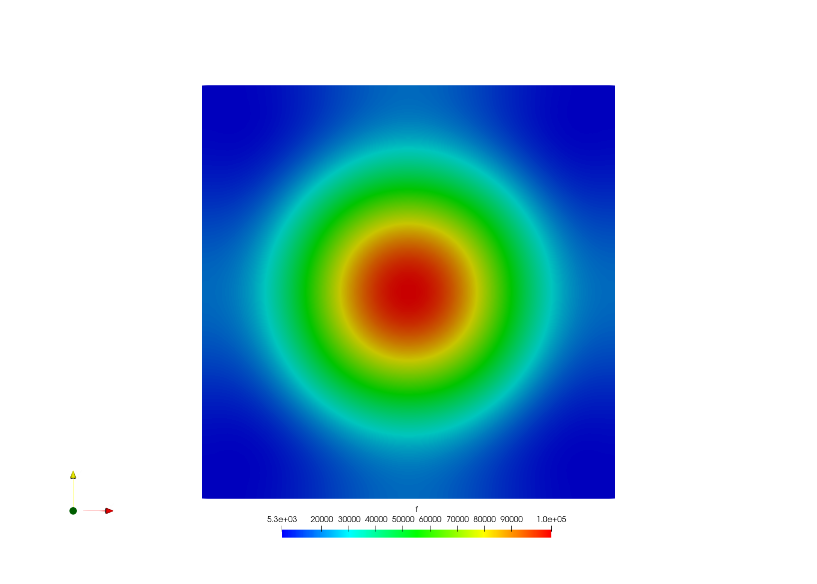
The resulting inverted source term
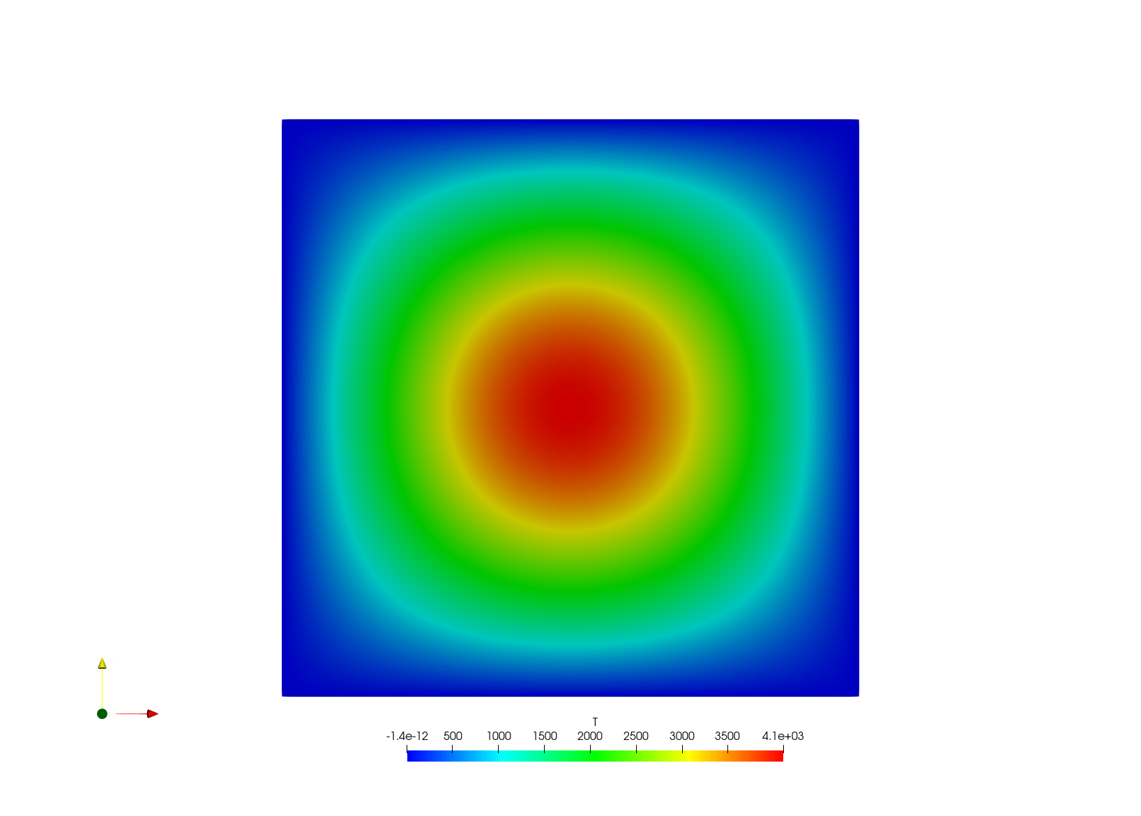
The resulting temperature field
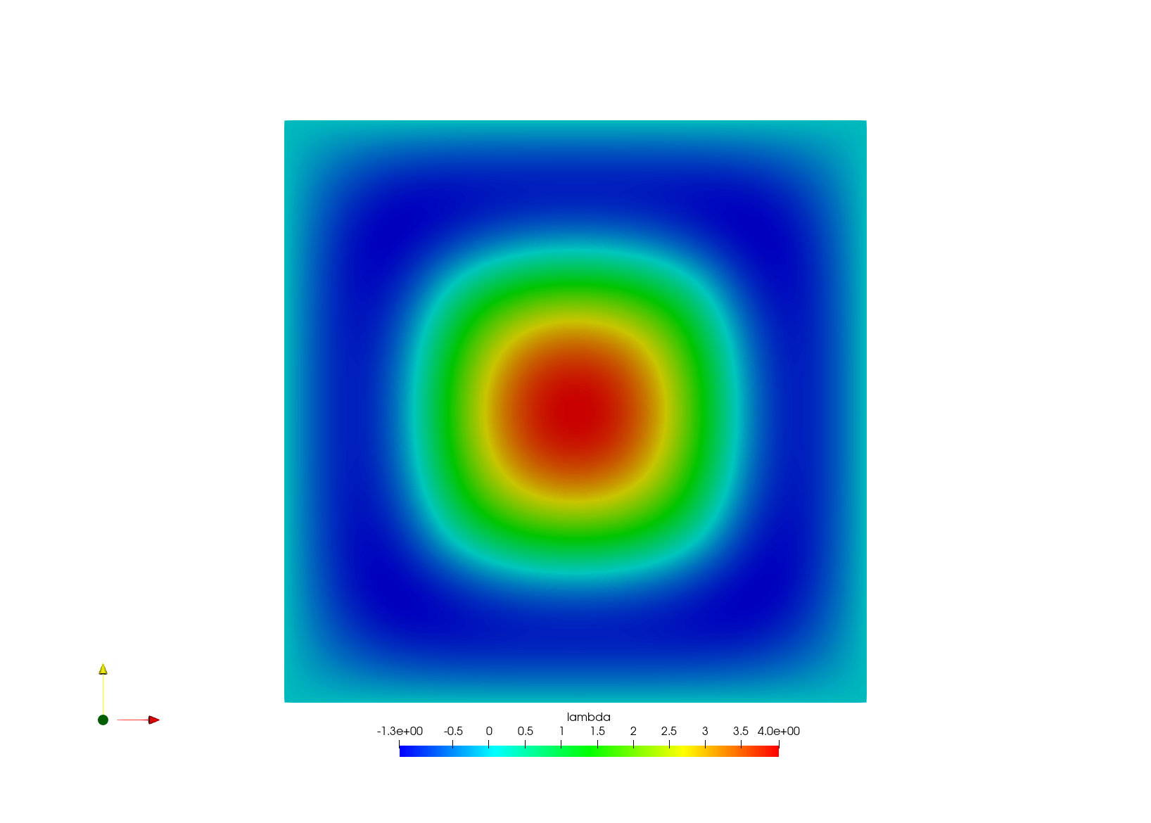
The value of the Lagrange multiplier
Page last modified: