Timestepping

This example addresses and illustrates the following topics:

• Definition of a simple parabolic equation
• Dirichlet boundary condition
• Definition of initial values
• Two time stepping procedures, namely
  • Implicit Euler method
  • Limex method
• Use of timing functions
• Output of the result for gnuplot, .vtk and as time series

and can be found at not available for public yet https://gitlab.com/Kaskade7 under tutorials/timedependentproblem. Execution of tutorials is described under Running the tutorials in section Getting Started/Installation.

Introduction

This tutorial program solves a parabolic heat equation with Dirichlet boundary condition and an initial value condition by the use of two different time integration methods. It shows the definition of an initial value, the implementation of the time integration step, the use of timing methods to keep track on computation time and the output of time dependent results. In addition, we present some extension possibilities and show the results of this tutorial example.

Mathematical model

Motivation

This tutorial deals with a parabolic problem of the form \[ c \frac{\partial u}{\partial t} - \nabla \cdot (\kappa \nabla u) = f \quad x\text{ in } \Omega, 0 < t \leq T \] in the 2-dimensional region \( \Omega \) with Dirichlet boundary condition on the boundary \( \Gamma \) \[ u = u_b \quad \text{on } \Gamma = \partial \Omega \] and initial condition \[ u = u_0 \quad \text{on } \Omega \text{ for } t=0. \] After formulation as a variational problem and Galerkin discretization, the problem can be stated as a system of ODEs by \[ B\dot u = Au - f \] with stiffness matrix \( A = \bigl( a(\varphi_i,\varphi_j)\bigr) _{i,j=1}^N \), \( a(\varphi_i,\varphi_j) = \int_\Omega \kappa \nabla \varphi_i \nabla \varphi_j dx \) and mass matrix \( B = \bigl((\varphi_i,\varphi_j)\bigr)_{i,j}^N \), \( (\varphi_i,\varphi_j) = \int_\Omega \varphi_i \varphi_j dx \).

The moving source example used for this tutorial shows a circulating moving source on a quadratic 2-dimensional unit grid.

With \( \kappa=1 \) and \( c=1 \) and the use of \( p = x_1 - 0.25(2+\sin(\pi t)) \) and \( q = x_2 - 0.25(2+\cos(\pi t)) \) the PDE from above is implemented with the following parameters:

Initial condition \[ u_0 = 0.8\exp(-80((x_1-0.5)^2 + (x_2-0.75)^2)) \] Boundary condition \[ u_b = 0.8\exp(-80(p^2 + q^2)) \] Source term \[ f = u_b(-25600(p^2+q^2) + 320 + 40\pi (p \cos(\pi t) - q \sin(\pi t))) \]

Time discretization: Linearly implicit Euler

From the general formulation with constant matrix \( B \) in section linearly implicit Euler \[ (B-\tau L’(u_0))\delta u^k = \tau L(u^k) \] we can deduct the specific formulation for our tutorial example with the residual as functional \( L(u) := Au-f \) \[ (B-\tau A)\delta u^k = \tau (Au^k-f). \] with the displacement \( \delta u^k = u^{k+1}-u^k\). One solution step to solve this system of ODEs could then be performed by a direct inverse operation (as the simplest method among others) \[ \delta u^k = (B-\tau A)^{-1}\tau (Au^k-f) \] resulting in the new iterate \( u^{k+1} = u^k + \delta u^k \).

LIMEX: Extrapolation method for linearly-implicit Euler

The Limex implementation in this tutorial example relies on the theory provided in section LIMEX. With basic stepsize \( H \) and definition of stepsizes \( \tau_j = \frac{H}{n_j} \) for the harmonic sequence \( n_j = 1,2,3, … \) we obtain different numerical solutions \( T_{j,1} \) at points \( (t_0 + H) \) by applying \( n_j \) steps of the linearly implicit Euler method \( \delta u^k = (B-\tau A)^{-1}\tau (Au^k-f) \).

In our tutorial example, we use extrapolation order 2. Hence, \( j_{max} = order+1 \), since in contrast to the pseudocode where \( j \) runs from 1 to \( j_{max} \), we loop over \( j \) from 0 to 2. To cancel out the higher order terms in the asymptotic expansion of the error of one basic approximation step, we set \( \gamma = 1 \). Then, the extrapolation formula of Aitken-Neville becomes \[ T_{j,k} = T_{j,k-1} + \frac{T_{j,k-1}-T_{j-1,k-1}}{\frac{n_j}{n_{j-k+1}}-1}, \qquad k=1,\ldots,j. \]

The extrapolation tableau with the linearly implicit Euler method as base method for LIMEX and extrapolation order 2 is given by \[ \begin{aligned} &T_{1,1} \\ &T_{2,1} && T_{2,2} \\ &T_{3,1} && T_{3,2} && T_{3,3} \end{aligned} \] where \( T_{1,1}, T_{2,1}, T_{3,1} \) correspond to order p from linearly implicit Euler. After a LIMEX step is performed, stepsize and order control is carried out by calculation of the temporal errors. Using the formula for setting a new basic stepsize provided in the theory section with \( p_j = j_{max}+1 = (\mathrm{order}+1) +1 = \mathrm{order}+2 \) and with \( \rho = 0.5 \): \[ H_{new} = \sqrt[\mathrm{order}+2]{0.5 \frac{\mathrm{eps}}{\epsilon}} H \] To prevent the stepsize factor from growing or shrinking too much, the factor \( \sqrt[\mathrm{order}+2]{0.5 \frac{\mathrm{eps}}{\epsilon}} \) gets bounded to 0.5 from below and 1.33 from above.

Deriving the domain and boundary caches

The domain cache with d1 and d2 defines the functions for assembly of mass and stiffness matrix and the right-hand side. Consider d0 as the domain part F of the variational functional of the elliptic equation (see section Variational functionals), derived by discretizing our parabolic equation: \[ \text{d0: } F(u) = -\frac{1}{2}\kappa u^2 + fu. \] Then, the caches d1 and d2 are calculated by the first and second Fréchet derivative in directon v and w of d0: \[ \begin{aligned} &\text{d1: } F’(u)[v] = -\kappa \nabla u \cdot \nabla v + fv \\ &\text{d2: } F’’(u)[v,w] = -\kappa \nabla v \cdot \nabla w \end{aligned} \] As it can be seen directly, the cache d2 resembles the stiffness matrix \( A \), while d1 is the right-hand side \( Au-f \).

The boundary condition is implemented in the boundary cache by the Dirichlet penalty approach. Here, we define a penalty parameter \(\epsilon \rightarrow \infty\) and define the boundary integral as \( \int_\Gamma \frac{\epsilon}{2}(u-u_b)^2 dS \) in the variational functional. Consider d0 as the boundary part G of the variational functional: \[ \text{d0: } G(u) = \epsilon (u-u_b)^2. \] Then, the d1 and d2 caches are calculated again by the first and second Fréchet derivative in directon v and w of d0: \[ \begin{aligned} &\text{d1: } G’(u)[v] = \epsilon(u-u_b)v \\ &\text{d2: } G’’(u)[v,w] = \epsilon vw \end{aligned} \]

Treatment of mass matrix

The mass matrix is built separately in the cache b2. Starting from \( \frac{1}{2} c u^2 \) after discretization and formulation in the variational functional, the b2 domain cache is again the second Fréchet derivative and simply defined as \[ \text{b2: } B’’(u)[v,w] = cvw \] The b2 boundary cache is set to zero.

Source code documentation

Overall structure of the tutorial program code

do we need all of the includes or are some of them redundant? Usual list of header files used in this tutorial:

#include <iostream>
#include <bits/stdc++.h>
#include <iostream>
#include <filesystem>
#include <sys/stat.h>
#include <sys/types.h>

#include <boost/timer/timer.hpp>            // for use of cpu timer

#include "dune/grid/config.h"               // in dune libraries
#include "dune/grid/uggrid.hh"              // in dune libraries

#include "fem/gridmanager.hh"
#include "fem/lagrangespace.hh"

#include "io/vtk.hh"                        // input/output methods
#include "io/vtkreader.hh"
#include "io/gnuplot.hh"

#include "timestepping/limexWithoutJens.hh" // limex with embedded error estimation
#include "utilities/gridGeneration.hh"      // create unit squares and cubes
#include "utilities/kaskopt.hh"             // for command line option parsing
#include "timestepping/semieuler.hh"        // define weak formulation for semi implicit euler

using namespace Kaskade;

#include "integrate.hh"
#include "movingsource.hh"

The following steps define this tutorial program:

• creation of initial values
• setting up the spaces
• creating the grid
• defining the equation of our problem
• creating the assembler
• solving: time-stepping and assembly
• solution output

Classes and functions in detail

Setting up the equation

To define our problem equation in Kaskade, we use the class MovingSourceEquation. Then, the equation is defined in the main function by

using Equation = MovingSourceEquation<double,VariableSet>;
Equation Eq(c,kappa); // e.g. c capacity, kappa conductivity

The domain and boundary caches (see section Deriving the domain and boundary caches) are implemented in this class in the header file movingsource.hh, as well as evaluation methods, the source term and functionalities to get and set the parameters for heat conduction, heat capacity and so on. The caches are used by the assembler via the class SemiImplicitEulerStep to build the left-hand side of our problem (i.e. stiffness and mass matrix) and the right-hand side. To sum up, in the header file we implement

• our problem equation in class MovingSourceEquation
• the class DomainCache for domain caches d1, d2 and b2
• the class BoundaryCache for boundary caches d1, d2 and b2 and the penalty parameter
• evaluation methods in evaluateAt for e.g. the source term, the variables and their derivatives, etc.
• get and set parameters of the equation
• helper methods and structures for assembly, time integration and initial values

Domain cache: The right-hand side is built in d1, the stiffness matrix is built in d2:

    template<int row, int dim> 
    Dune::FieldVector<Scalar, TestVars::template Components<row>::m>
    d1 (VariationalArg<Scalar,dim> const& arg) const 
    {
      return -F.kappa*du*arg.derivative[0] + f*arg.value;
    }

    template<int row, int col, int dim> 
    Dune::FieldMatrix<Scalar, TestVars::template Components<row>::m, AnsatzVars::template Components<col>::m>
    d2 (VariationalArg<Scalar,dim> const &arg1, VariationalArg<Scalar,dim> const &arg2) const 
    {
      return -F.kappa*arg1.derivative[0]*arg2.derivative[0];
    }

The mass matrix is built in b2. Note: This cache is not directly evaluated by the assembler and requires the construction of a ParabolicEquation in the class SemiImplicitEulerStep. The b2 cache then gets evaluated by this proxy class and handed over to the assembler as d2.

    template<int row, int col, int dim> 
    Dune::FieldMatrix<Scalar, TestVars::template Components<row>::m, AnsatzVars::template Components<col>::m>
    b2 (VariationalArg<Scalar,dim> const &arg1, VariationalArg<Scalar,dim> const &arg2) const 
    {
      return F.c*arg1.value[0]*arg2.value[0];
    }

Boundary cache: The boundary conditions are implemented in the same way as the domain:

    template<int row, int dim> 
    Dune::FieldVector<Scalar, TestVars::template Components<row>::m>
    d1 (VariationalArg<Scalar,dim> const& arg) const 
    {
      return penalty*(u-ub)*arg.value[0];
    }
    template<int row, int col, int dim> 
    Dune::FieldMatrix<Scalar, TestVars::template Components<row>::m, AnsatzVars::template Components<col>::m>
    d2 (VariationalArg<Scalar,dim> const &arg1, VariationalArg<Scalar,dim> const &arg2) const 
    {
      return penalty*arg1.value*arg2.value;
    }
    template<int row, int col, int dim> 
    Dune::FieldMatrix<Scalar, TestVars::template Components<row>::m, AnsatzVars::template Components<col>::m>
    b2 (VariationalArg<Scalar,dim> const &arg1, VariationalArg<Scalar,dim> const &arg2) const 
    {
      return 0;
    }

The penalty parameter has to be defined as well. It is set to a very large number, here 10⁹:

    void moveTo(FaceIterator const& entity)
    {
      e = &entity;
      penalty = 1.0e9; // for Dirichlet boundary condition
    }

We can provide additional information about our problem by defining structures struct for the assembly. In this example our mass matrix \( B \) does not depend on \( u \). Therefore, we set the parameter constant = true in B2. Further, our stiffness matrix is symmetric, same holds for the mass matrix, and we set the parameter symmetric = true in D2 and B2. Other parameters depending on the problem definition can be added to B2 such as mass lumping via lumping = true, if required and applicable:

template <int row>
  struct D1: public FunctionalBase<WeakFormulation>::D1<row> 
  {
    static bool const present   = true;
    static bool const constant  = false;
  };

  template <int row, int col>
  struct D2: public FunctionalBase<WeakFormulation>::D2<row,col> 
  {
    static bool const present = true;
    static bool const symmetric = true;
    static bool const lumped = false;
  };

  template <int row, int col>
  struct B2 
  {
    static bool const present   = true;
    static bool const symmetric = true;
    static bool const constant  = true;
    static bool const lumped = false;
  };

Hint: It is possible as well to define a cache d0 for domain and boundary in the header file (not implemented in the tutorial) for a problem based on a variational functional. This d0 cache can be accessed via the assembler. Then, one could use this

Scalar
  d0() const 
  {
    return -(F.kappa*du*du)/2 + f*u;
  }

and the corresponding formulation for the boundary condition in the boudary cache to evaluate the functional in our main program by calling

double val = assembler.functional();

Initial value definition

is this stuff correct/clear? In the Galerkin method, our initial condition \(u(0,x)=u_b(x) \) is expressed as \( u_b(x) = \sum_{j=1}^N u_{0,j} \varphi_j \). Hence, we have to assure that the initial condition \( u_b \) is set properly by defining the values \( u_{0,j} \) in the finite element mesh as so called “function space elements”. Since we cannot do this manually for all nodes, the initial values are interpolated and assigned with help of some functions in Kaskade 7 that implement the basic concepts:

• the new user-defined data type InitialValue
• the user-defined method scaleInitialValue in the header file
• the basic Kaskade 7 interpolation method interpolateGloballyWeak
• the Kaskade 7 concepts of WeakFunctionView and FunctionSpaceElement

In the main file, the initial value \( u_b(x) \) is set by the use of the new user-defined data type InitialValue. Here in a 2 dimensional setting, the initial value could be set for example to x*val+y:

struct InitialValue 
{
  static int const components = 1;
  using ValueType = Dune::FieldVector<Scalar,components>;

  InitialValue(int c, double v): component(c), val(v) {} // constructor
  
  template <class Cell> int order(Cell const&) const { return std::numeric_limits<int>::max(); }
  template <class Cell>
  ValueType value(Cell const& cell,
                  Dune::FieldVector<typename Cell::Geometry::ctype,Cell::dimension> const& localCoordinate) const 
  {
    Dune::FieldVector<typename Cell::Geometry::ctype,Cell::Geometry::coorddimension> x = cell.geometry().global(localCoordinate);

    return x[0]*val+x[1]; // example with a value set by the user on construction
  }

private:
  int component;
  double val;
};

Then, the initial value of the equation is assigned by method scaleInitialValue, defined in the header file, which transforms the values into proper finite element iterates:

  using Equation = MovingSourceEquation<double,VariableSet>;
  
  Equation Eq(c,kappa); // e.g. c capacity, kappa conductivity

  Eq.scaleInitialValue<0>(InitialValue(0,273.15),x); // VariableSet x, initial value 273.15

The definition in the header by using the lambda function makeWeakFunctionView file looks as follows:

template <int row, class WeakFunctionView>
  void scaleInitialValue(WeakFunctionView const& u0, typename AnsatzVars::VariableSet& u) const 
  {
    interpolateGloballyWeak(boost::fusion::at_c<row>(u.data),makeWeakFunctionView([u0](auto const& cell, auto const& xi) { auto x = cell.geometry().global(xi); return u0.value(cell,xi); }));
  }

Here, the interpolateGloballyWeak method makes it possible to transform a WeakFunctionView to a FunctionSpaceElement by interpolation. A WeakFunctionView is basically a class that supports efficient evaluation by cell and local coordinate (at the evaluation point in the cell), whileas a FunctionView is a function that supports evaluation by an evaluator.

An alternative is using a newly defined data type ScaledFunction why? advantages? for creating interpolates by interpolateGloballyWeak

  interpolateGloballyWeak<Volume>(boost::fusion::at_c<row>(u.data),ScaledFunction<WeakFunctionView>(true,u0,*this));

Now, we have successfully transformed our initial value to a FunctionSpaceElement for calculation, which is simply the representation of a component of the underlying finite element function space.

Implementing the Euler steps

The class SemiImplicitEulerStep defines the weak formulation of this stationary elliptic problem, resulting from time discretization of a parabolic PDE, and provides the implementation of \( B-\tau A \) and right hand side \( \tau (Au^k-f) \) for assembly. The matrices \( A \), \( B \) and the vector \( (Au^k-f) \) are assembled based on the d1, d2 and b2 caches in the corresponding header file movingsource.hh of the parabolic equation, see section Setting up the equation.

The class SemiLinearizationAt, a proxy class for the linearization of semi-linear time stepping schemes, requires the second linearization point \( u_0 \) which is used to compute the Jacobian denoted by \( L’ \) occuring in \[ B \dot u - L’ u = L(u) - L’ u. \]

for (int i=0; i<MaxIter; ++i) 
    {
      SemiImplicitEulerStep<Equation> eq(&Eq,dt);
      double const tau = dt;
      eq.setTau(tau);
      
      assembler.assemble(Linearization(eq,x,x,dx));
      AssembledGalerkinOperator<Assembler> A(assembler);

      auto step = variableSet.zeroCoefficientVector();
      auto rhs = assembler.rhs();
      
      directInverseOperator(A,DirectType::UMFPACK,MatrixProperties::GENERAL).applyscaleadd(1,rhs,step);
      component<0>(x) += component<0>(step);
      Eq.setTime(Eq.time()+dt);
    }

where

  using Linearization = SemiLinearizationAt<SemiImplicitEulerStep<Equation>>;
  using Assembler = VariationalFunctionalAssembler<Linearization>;

In each step, the system is solved by a simple direct inverse operation and the new iterate \( u^{k+1} = u^k +\delta u^k \) is calculated, until the maximum number MaxIter of desired iterations is reached.

Perform time integration with LIMEX

Time-integration according to the Limex theory section and Limex tutorial section is performed within the header file integrate.hh which calls the Limex from timestepping/limexWithoutJens.hh. The basic stepsize for the current iteration is set and followed by one step of Limex. Afterwards, the temporal error is estimated for this step and used to calculate the next basic stepsize. Hence, this is an adaptive method for calculating good basic stepsizes.

The procedure is as follows:

• construct LIMEX integrator for time integration,
• loop over number of desired steps to perform time stepping with LIMEX and
• adapt basic stepsize by estimated errors after each step.

First, the LIMEX integrator has to be constructed, templated by our PDE equation and based on the grid, the specific equation, the variables and the choice of a direct or iterative solver and a preconditioner:

Limex<Equation> limex(gridManager,eq,variableSet,directType,PrecondType::ILUK,verbosity);

The steps of the time integration then are performed as follows:

for (steps=0; !done && steps<maxSteps; ++steps)
{
  [...]

  dt *= factor; // set new basic stepsize
  dx = limex.step(x,dt,extrapolOrder,tolX); // perform one step of LIMEX
  std::vector<std::pair<double,double> > errors = limex.estimateError(x,extrapolOrder,extrapolOrder-1); // errors in time

  [adapt stepsize]
}

Calculation of the factor for the next basic stepsize relies on the subdiagonal error, the desired accuracy, a safety factor and the extrapolation order:

dt *= factor;

[limex step with new dt]

std::vector<std::pair<double,double> > errors = limex.estimateError(x,extrapolOrder,extrapolOrder-1); // subdiagonal errors
err = 0;
for (int i=0; i<errors.size(); ++i)
  err = std::max(err, errors[i].first/(tolT[i].first+tolT[i].second*errors[i].second)); // subdiagonal errors and accuracy

factor = std::pow(0.5/err,1./(extrapolOrder+2)); // safety factor = 0.5
factor = std::max(0.5,std::min(factor,1.33)); // bound factor from above and below

Here, errors = limex.estimateError(x,p,p-1) provides the subdiagonal errors and the current state such that for each i, errors[i].first gives the subdiagonal error \( |T_{p,p}-T_{p,p-1}| \) with \( p \) as the extrapolation order and errors[i].second gives the current state \( u \). If our problem is defined in more than on variable or solution component \( u \), the i iterates over the number of variables/solution components to find the largest overall error. Then, the quotient \( \mathrm{err} = \frac{\epsilon}{\mathrm{eps}} \) is calculated. The update factor for the new basic stepsize \( H_{new} \) is calculated with safety factor \( 0.5 \), yielding \( \frac{0.5}{\mathrm{err}} = 0.5\frac{\mathrm{eps}}{\epsilon} \) to the power of \( \frac{1}{\mathrm{order}+2 } \). To prevent the stepsize factor from growing or shrinking too much, the factor gets bounded to \( 0.5 \) from below and \( 1.33 \) from above.

One step of Limex computes a state increment dx that advances the given current state x in time. Setting an extrapolation order of zero simply corresponds to the linearly implicit Euler without calculation of higher order approximations. The for-loop in i calculates the \( T_{j,1} \), while the propagation loop over j calculates the higher-order approximations and the \( T_{j,j} \) during the push_back into the extrapolation tableau. This happens in timestepping/limexWithoutJens.hh, where the LIMEX algorithm is implemented as follows:

State const& step(State const& x, double dt, int order, std::vector<std::pair<double,double>> const& tolX)
{
  for (int i=0; i<=extrapolationorder; ++i)
  {
    [calculate step fractions tau]
    // mesh adaption loop if spatial error too large, expressed by variable "accurate"
    do { 
      [assemble current system]
      [solve system yielding increment dx]
      [perform mesh adaption] // only if in first stage of Euler step i=0
    } while (!accurate);
    [set new state increment, dxsum = dx]
    
    // propagation for tableau
    if (extrapolationorder==0) 
    {
      [insert dxsum into extrapolation tableau] // theory: T_1,1
      [return last state increment]
    }
    else
    {
      for (int j=1; j<=i; ++j)
      {
        [assemble system with new rhs x+dx]
        [solve system]
        [add new state increment dx to previous one, dxsum += dx]
      }
    }
    [insert dxsum into extrapolation tableau] // theory: T_j,1
  }
  [return last state increment] // theory: T_j,j
}

The class ExtrapolationTableau handles the calculation of the higher-order approximations \( T_{j,k} \) and \( T_{j,j} \) by the Aitken-Neville formula during insertion into the tableau by extrap.push_back(dxsum,stepFractions[i]).

Estimation of errors

Measure program execution times: Timings vs. Boost Timer

Sometimes it is useful to know how long a program takes for execution. Such timing information may be divided into wall time, user CPU time and system CPU time. Wall time is the time that a clock on the wall would measure between start of the process and now. The amount of time spent in user code (your program code and code from third-party libraries) is the user CPU time, while the amount of time spent in kernel code (code that is part of the operating system) is the system CPU time. Units are in seconds. On a single core machine, wall time will be always greater than CPU time. Using multi-core machines and multi-threaded programs, this can cause multiple CPU seconds of effort per second of elapsed wall time. The two methods presented here base on the implementation of

• boost::timer::cpu_timer from boost libraries and
• the Timings class, implemented in Kaskade 7.

A handy tool is the boost::timer::cpu_timer from boost libraries. A detailed explanation can be found here: Boost Timer. In this tutorial example, a timer for the execution of the whole program is set and accompanied by timers for assembly and solution within the semi-implicit Euler method. When the timer object is created, it starts the time measurement.

boost::timer::cpu_timer totalTimer;
std::cout << "Start moving source tutorial program" << std::endl;

[program code]

std::cout << "Total cpu time: " << totalTimer.format() << "\n";
std::cout << "End moving source tutorial program" << std::endl;

Calling format() at any point to get elapsed time as wall, user and system time. Using the member function elapsed() instead lets you chose between output of only wall, user or system time. Timers can be started, stopped and resumed. Calling start() restarts the timer from zero. To measure e.g. the time used for assembly over the whole loop, create a variable assemblyTime and sum up the elapsed time:

double assemblyTime;
for (int i=0; i<MaxIter; ++i) // time integration loop
{
  [...]
  timer.start();
  assembler.assemble(Linearization(eq,x,x,dx));
  assemblyTime += (double)(timer.elapsed().user)/1e9; // measured in user time
  [...]
}
std::cerr << "Euler: " << assemblyTime << "s assembly\n" << std::flush;

The elapsed time is here measured in user time, but could as well be measured in wall time timer.elapsed().wall, system time timer.elapsed().system or all three together.

This can be done for other parts of the program in the same manner, as shown for the solutionTime in the Euler section, i.e. the time the direct inverse operator takes to solve the system.

Another option is the use of the Timings class, implemented in Kaskade 7. It is used to gather and report execution times information for nested program parts. As well, for timing investigation in multithreaded computations, the class TaskTiming can be used, yielding a gnuplot file to visualize task durations. After creating of an instance of Timings, the part of interest has to be wrapped in start() and stop() and labeled by a certain name. To set the timer back to zero, call clear(). This could look as follows:

Timings& timings = Timings::instance();

for (int i=0; i<MaxIter; ++i) // time integration loop
{
  [...]
  timings.start("matrix assembly");
  assembler.assemble(Linearization(eq,x,x,dx));
  timings.stop("matrix assembly");
  [...]
  std::cout << "Setup:" << timings;
  timings.clear(); 
}

This procedure gives you a detailed overview of the execution times of the processes, assigned to their given names and arranged in the order of their creation.

Writing .gnu output

For instant visualization or creating figures for publications with gnuplot, Kaskade 7 provides the possibility to directly write output into a data file. This file can be instantly processed by a predefined gnuplot script file of the same name. Instead of calling gnuplot and plotting commands manually one after another, the script file allows for a sequence of commands to draw a figure. There are tutorials available online for creation of such scripts. Documentation and FAQ for gnuplot can be found on the gnuplot website www.gnuplot.info. Two different ideas of what to plot are implemented in this tutorial example.

In the semi-implicit Euler loop, a data file function.data is written only at the last time step of the calculation.

writeGnuplotFile(x,"function"); // write gnuplot output and call gnuplot script file

Afterwards, the script function.gnu is executed. First, a 3d plot is created and saved as .png image file, showing the result at end time T. Second, a 2d heat map of the same data is created and saved as .png, too.

In the LIMEX integration method, data is written as time series and a .gif is created and stored by a gnuplot script called function40.equidist.gnu, showing the moving source. After termination of the program, the data files may be deleted (among others) by the usual make clean command. Since the LIMEX deals with adaptive timestepping, the data for the animation has to be interpolated to equidistant time steps:

double outTime = eq.time()+outInterval; // outInterval is the write interval, here = 0.05
[...]
while (outTime <= eq.time()+dt) {
  typename VariableSet::VariableSet z(x);
  z.axpy((outTime-eq.time())/dt,dx); // interpolation
  writeGnuplotFile(z,"function"+paddedString(ceil(outTime*200)/10,2)+".equidist"); // write gnuplot output and call gnuplot script which does not exist, so ignore the error messages
  outTime += outInterval;
    }

(Note the rounding trick at ceil(outTime*200)/10 instead of ceil(outTime*20) - this is necessary due to floating-point arithmetic on a computer.) Calling gnuplot function-show.gnu in the console will open subsequently two windows, showing the same figures as the saved ones before. To get rid of the time series data files and clear the graph folder, call make clean to remove these files.

As well, it is possible to write data at a certain sample position into a gnu data file and use this afterwards for plotting with e.g. gnuplot or Matlab. This is demonstrated in the semi-implicit Euler loop and in the LIMEX integration method by the use of a static std::ofstream. Data at a specified sample position is written into a data file together with its timestep.

Dune::FieldVector<double,2> samplePos(0); 
samplePos[0] = 0.5;
samplePos[1] = 0.2;
[...]
static std::ofstream sampleOut("samplepositionEuler.dat"); // data file: output of result at sample position
sampleOut << std::to_string(Eq.time()) << ' '  << ' ' <<  component<0>(x).value(samplePos)[0] << std::endl;

This is especially useful for comparing measurement data taken at a certain sample position with simulated data and generating measurement curves.

Writing time series in .vtk format

Results

Some of these results are generated directly within this tutorial example, while further results are provided to show different aspects of the solution, the behavior of the integration methods and the evolution of errors during the calculation. All of the data for these results was generated without modifying the code of this example.

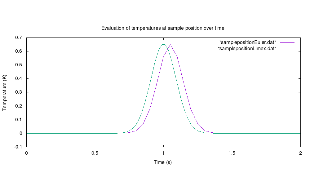
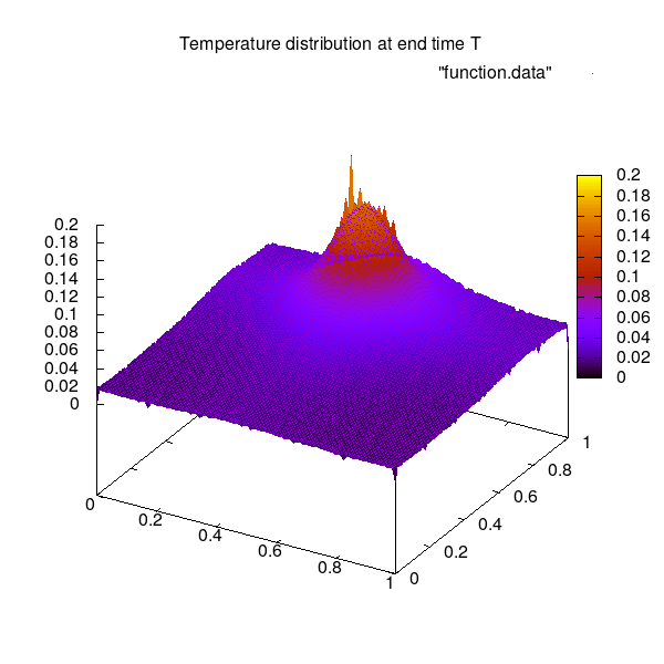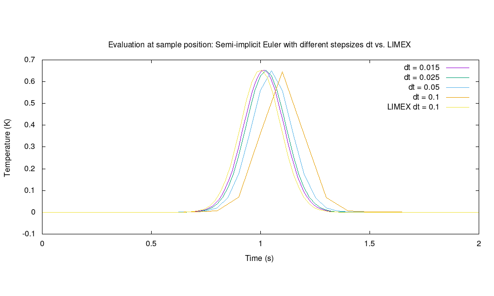
The moving source as 2D heat map over the unit square: 3D representation of the solution at end time T: Evaluation of temperatures at a specific sample position within the unit square for semi-implicit Euler with basic stepsize dt = 0.05 and LIMEX with dt = 0.025: Evaluation of temperatures at a specific sample position within the unit square for semi-implicit Euler with decreasing basic stepsizes vs. LIMEX:

Possibilities for extension