More Examples
This section presents a set of examples which are not covered in detail in the previous sections. The examples can be found in the tutorial folder in Kaskade 7.
Stationary heat transfer
This tutorial can be found at tutorial/stationary_heattransfer. It covers
- a stationary heat transfer problem in 2 or 3 dimensions on a simple square/cubic grid
- with source term,
- Dirichlet and Neumann boundary conditions on different parts of the boundary,
- use of boost::timer for timing,
- the possibility to choose between direct and iterative solution plus preconditioners of the linear systems
- and .vtk output.
The PDE is given by
\[ \begin{aligned} -\nabla \cdot (\kappa \nabla u) + qu &= f &&\quad x \in \Omega \\ \kappa \frac{\partial u}{\partial n} &= 0 &&\quad \text{on } \Gamma_1 \\ u &= u_b &&\quad \text{on } \Gamma_2 \end{aligned} \]
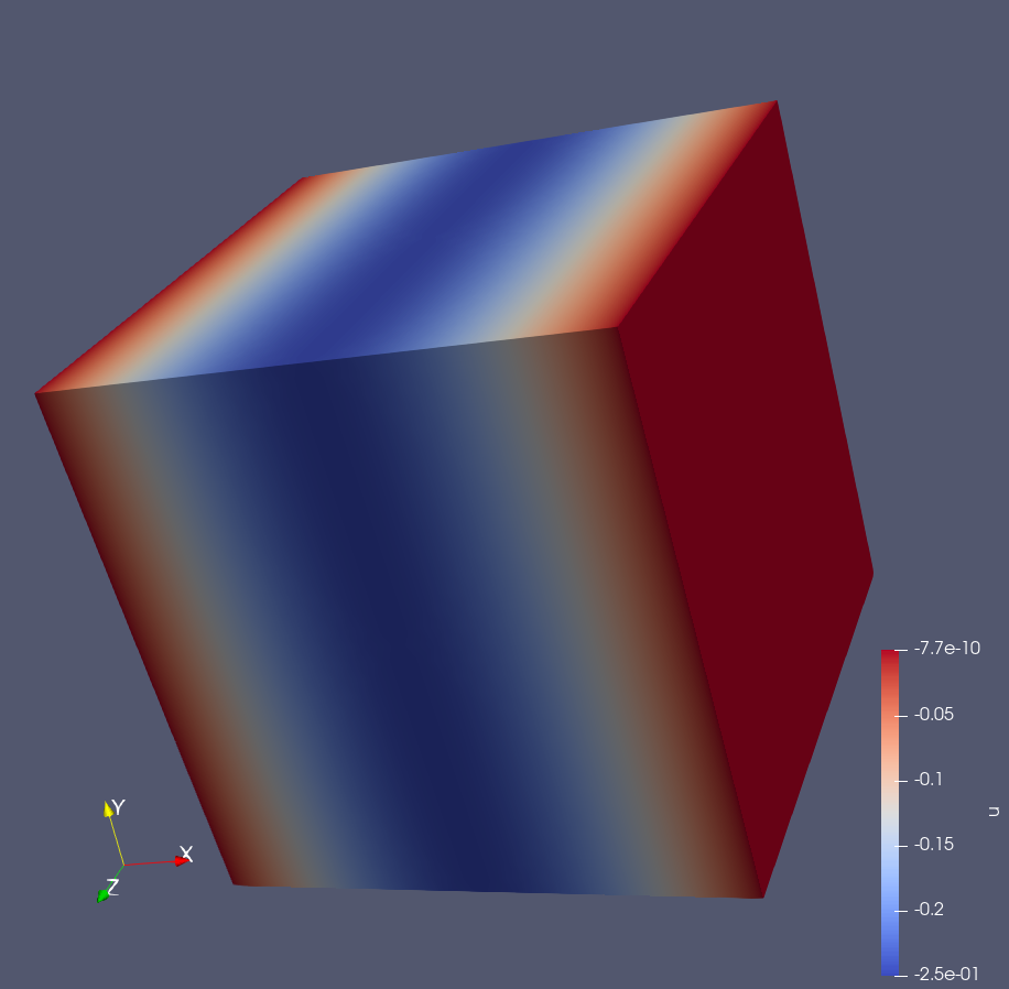
with \( \partial \Omega = \Gamma_1 \cup \Gamma_2 \), where \( \Gamma_1 = \{x_1=0,x_1=1\} \). The domain is the unit square or unit cube. These equations are implemented in heat.hh. For calculations, we set \( \kappa=1 \), \( q=1 \), \( u_b = 0 \) and the source \( f \) in a way such that \( u = x_1(x_1-1) e^{-(x_1-0.5)^2}\) is solution of the above PDE for \( x=(x_1,x_2) \in \Omega \) for dimension 2 or \( x=(x_1,x_2,x_3) \in \Omega \) for dimension 3:
template <class Evaluators>
void evaluateAt(LocalPosition<Grid> const& x, Evaluators const& evaluators)
{
  u  = data.template value<0>(evaluators);
  du = data.template derivative<0>(evaluators)[0];

  xglob = cell.geometry().global(x);

  double v, w, vX, vXX, wX, wXX, uXX;
  v   = xglob[0]*(xglob[0] - 1);
  w   = exp(-(xglob[0] - 0.5)*(xglob[0] - 0.5));

  vX  =  2*xglob[0] - 1;
  vXX =  2;
  wX  = -2*(xglob[0] - 0.5)*w;
  wXX = -2*w - 2*(xglob[0] - 0.5)*wX;

  uXX = vXX*w + 2*vX*wX + v*wXX;
  f   = -F.kappa*uXX + F.q*v*w;
}
template<int row, int col, int dim>
  Dune::FieldMatrix<Scalar, TestVars::template Components<row>::m, AnsatzVars::template Components<col>::m>
  d2 (VariationalArg<Scalar,dim> const &arg1, VariationalArg<Scalar,dim> const &arg2) const
  {
    if ( (xglob[0]<=1e-12) || (xglob[0]>=(1-1e-12)) )
      return penalty*arg1.value*arg2.value;
    else return 0.0;
  }
Direct or iterative solver timing functions for assembly, solution, etc.
Output as .vtk for visualization or gnuplot (3D):
Instationary Navier-Stokes equation
This tutorial can be found at tutorial/instationary_NavierStokes It deals with the
- instationary 2D driven cavity problem for incompressible fluids
- on the unit square,
- governed by the Navier-Stokes equations
- with Dirichlet boundary condition,
- inital value definition,
- definition of pressure and velocity spaces and
- solution by LIMEX for time integration.
The PDE is given by
\[ \begin{aligned} \frac{\partial u}{\partial t}-\mu \Delta u + (u\cdot \nabla)u+\frac{1}{\rho} \nabla p &= 0 &&\quad (x,y) \in \Omega \\ \nabla \cdot u &= 0 &&\quad (x,y) \in \Omega \\ u(x,y,t) &= -1 &&\quad \text{on } \partial \Omega|_{y=1} \\ u(x,y,t) &= 0 &&\quad \text{elsewhere on } \partial \Omega \\ u(x,y,0) &= 0 &&\quad (x,y) \in \Omega \end{aligned} \]
with velocity \( u=\bigl( u_1(x,y,t), u_2(x,y,t) \bigr)^T \), pressure \( p=p(x,y,t) \), density of the fluid \( \rho \), kinematic viscosity \( \mu \). The domain is the unit square \( \Omega = [0,1] \times [0,1] \). For incompressible flows, no explicit boundary conditions for the pressure must be given.
using VariableDescriptions = vector<Variable<SpaceIndex<1>,Components<2>,VariableId<uIdx>>,
                                    Variable<SpaceIndex<0>,Components<1>,VariableId<pIdx>>>;
[...]
H1Space pressureSpace(gridManager,gridManager.grid().leafGridView(),order-1); // order for pressure space is (order-1)
H1Space velocitySpace(gridManager,gridManager.grid().leafGridView(),order);
Embedded error estimation
For the example in tutorial/Embedded_errorEstimation, we consider
- the stationary heat equation in 2D or 3D
- on a unit square domain
- with source term representing a peak source,
- Dirichlet boundary conditions,
- a discretization based on P2 elements
- and the control of the discretization error by an embedded error estimation.
This equation \[ \begin{aligned} -\nabla \cdot (\nabla u) &= f(x) &&\quad x\in \Omega \\ u &= u_b(x) &&\quad \text{on } \partial \Omega \end{aligned} \] for \( x=(x_1,x_2) \) or \( x=(x_1,x_2,x_3) \) is treated in the same way as the stationary heat transfer problem (for implementation details see as well: Laplace equation). The right-hand side is determined in a way such that \[ u=x_1x_2(x_1-1)(x_2-1)e^{-100((x_1-0.5)^2+(x_2-0.5)^2)} \] is the solution of the equation in 2D. In 3D, the equation reads analogously. We set \( u_b(x) = 0 \) for homogeneous boundary conditions. We now control the discretization error by an error estimation, where the estimator provides information about the global and local error (read more in section Adaptivity). The local estimation is used to refine the mesh where the estimated error exceeds a certain prescribed threshold. If the global error indicates sufficient accuracy, the mesh adaption procedure stops.
// perform local mesh adaption while local error tolerance not "accurate", i.e. not met
do{
  [... solve equation ...]
  x.data = solution.data;

  // embedded error estimation:

  VariableSet::VariableSet e = x;
  projectHierarchically(variableSet,e);
  e -= x; // representation of the error

  accurate = embeddedErrorEstimator(variableSet,e,x,IdentityScaling(),tol,gridManager,verbosity); // returns true if the error is below the tolerance and the mesh hat not been refined, otherwise false
  nnz = assembler.nnz(0,1,0,1,onlyLowerTriangle);
  size_t size = variableSet.degreesOfFreedom(0,1); // get current number of dof if the mesh has been refined

} while (!accurate)
Hierarchical error estimation
We consider for tutorial/HB_errorEstimation the same problem as in example embedded error estimation. The difference is the usage of P1 elements, i.e. linear finite elements instead of P2 elements. Again, we control the discretization error by an error estimation, providing information about the global and the local error. But since the embedded error estimator is not applicable for linear finite elements, we use a hierarchic error estimator instead. To solve the defect equation for the error later, we create an higher order extension space for the application of the a posteriori error estimate
using H1ExSpaces = boost::fusion::vector<H1Space<Grid> const*,H1HierarchicExtensionSpace<Grid> const*>;
[...]
H1HierarchicExtensionSpace<Grid> spaceEx(gridManager,gridManager.grid().leafGridView(), order+1);
H1ExSpaces exSpaces(&temperatureSpace,&spaceEx);
accompanied by the according variable sets, coefficient vectors, assembler and so on. The procedure then is shown in section Adaptivity.
Aliev-Panfilov equation
Models of cardiac electrophysiology to simulate tissue and organ activities are often very complex. To address this, simplified models such as the Aliev-Panfilov model (see AlievPanfilov1996) were developed to reduce model complexity while providing necessary details of cardiac functions. In this tutorial at tutorial/cardio we show
- the Aliev-Panfilov equations with
- zero initial or excitation? and Neumann boundary condition,
- time-integration by Limex
- and output as .vtu (Paraview) and .am (Amira) files.
The equations to describe the fast resp. slow processes are defined in two variables as \[ \begin{aligned} \frac{\partial u}{\partial t} &= \kappa \frac{\partial^2 u}{\partial x^2}-g_a u (u-a)(u-1) - uv \\ \frac{\partial v}{\partial t} &= \epsilon(u,v) (-v- g_s u (u-a-1)) \\ \end{aligned} \] on a 3D domain with \( \epsilon(u,v)=\epsilon_0 + \frac{\mu_1 v}{u+\mu_2} \). Here, \( u \) is the transmembrane potential and \( v \) is the recovery variable that initiates repolarization.
Cardiac activities such as the initiation and upstroke of action potential are controlled by the first term. The parameters \( g_a, g_s \) are an excitation rate constant, \( \kappa \) is the conductivity which is determined by the electrical conductivity of myocardium. The parameter \( a \) is the threshold parameter related to the excitation threshold potential. The restitution properties of the action potential are determined by the term \( \epsilon(u,v) \) with restitution parameters \( \mu_1, \mu_2 \) and \( \epsilon_0 \). The system obeys no flux Neumann boundary conditions.
The parameters used in this tutorial are
kappa = 0.001;
a = 0.1;
gs = 8.0;
ga = 8.0;
mu1 = 0.07;
mu2 = 0.3;
eps1 = 0.01; // epsilon_0
The geometry is created by using the createCuboid method:
double dh = 0.1;
Dune::FieldVector<double,dim> c0(0.0), dc(0.0);
c0[0]=1.0; c0[1]=1.0; c0[2]=1.0;
dc[0]=1.0; dc[1]=1.0; dc[2]=0.1;
GridManager<Grid> gridManager( createCuboid<Grid>(c0,dc,dh,true) );
Assembly of the system of two variables is done within the d1 and d2 caches. Here, the right-hand sides (d1), stiffness (d2) and mass (b2) matrices get assembled in blocks via row and col indices, e.g. for d1 cache:
template<int row, int dim>
Dune::FieldVector<Scalar, TestVars::template Components<row>::m>
d1 (VariationalArg<Scalar,dim> const& arg) const
{
  if (row==uIdx) return -F.kappa*(du*arg.derivative[0]) + f(u,v)*arg.value + ex*arg.value;
  else if (row==vIdx) return g(u,v)*arg.value;
  assert("wrong index\n"==0);
  return 0;
}
with \( f(u,v) = -g_a u (u-a)(u-1)+uv \) and \( g(u,v) = \frac{1}{4}(\epsilon_0 +\frac{\mu_1 v}{u+\mu_2})(-v-g_s u(u-a-1)) \) and initial excitation ex modeled as
Scalar excitation(Position const& x) const
{
  Scalar Iapp = 0.0;

  // slab
  if(t<0.015)
    if ( (x[0]>=1.4) && (x[0]<=1.6) && (x[1]>=1.4) && (x[1]<=1.6) && (x[2]>=1.05) && (x[2]<=1.1) )
    {
      Iapp=10000.0*t;
      if (Iapp > 100.0) Iapp = 100.0;
    }
  return Iapp;
}
TODO include image/diagram
Stokes equation
We consider for the tutorial at tutorial/stokes the
- linear Stokes equations,
- describing the stationary 2D driven cavity problem for incompressible fluids
- on the unit square \( \Omega = [0,1]\times [0,1] \)
- solved either directly or by the Uzawa method.
\[ \begin{aligned} -\Delta u + \nabla p &= 0 && \quad (x,y) \in \Omega \\ \nabla \cdot u &= 0 && \quad (x,y) \in \Omega \\ u(x,y) &= -1 &&\quad \text{on } \partial \Omega|_{y=1} \\ u(x,y) &= 0 &&\quad \text{elsewhere on } \partial \Omega \end{aligned} \] with velocity \( u=u(x,y) \) and pressure \( p=p(x,y) \). We have to construct a velocity and a pressure space of different orders
H1Space pressureSpace(gridManager,gridManager.grid().leafGridView(),order-1);
H1Space velocitySpace(gridManager,gridManager.grid().leafGridView(),order);
SST pollution
This example is a model for the pollution of the statosphere by supersonic transport aircrafts (SST). It describes the interaction of chemical species O, O3, NO and NO2 along with a simple diffusion process. It can be found at tutorial/sst_pollution and deals with
- a stationary 2D model of diffusion
- with nonlinearities by using Newton’s method and the GIANT-GBIT package
- on the unit square
- with homogeneous Neumann boundary condition
- and with a default parameter file
default.json.
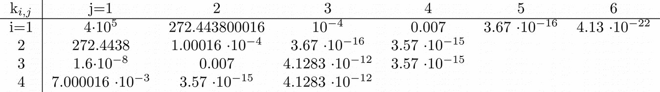
System of four equations
\[
\begin{aligned}
0 &= D\Delta u_1 + k_{1,1} - k_{1,2}u_1 +k_{1,3}u_2 + k_{1,4}u_4 - k_{1,5}u_1 u_2 - k_{1,6} u_1 u_4 \\
0 &= D\Delta u_2 + k_{2,1}u_1 - k_{2,2}u_2 + k_{2,3}u_1 u_2 - k_{2,4} u_2 u_3 \\
0 &= D\Delta u_3 - k_{3,1}u_3 + k_{3,2}u_4 + k_{3,3}u_1 u_4 - k_{3,4} u_2 u_3 + 800.0 + \text{SST} \\
0 &= D\Delta u_4 - k_{4,1}u_4 + k_{4,2}u_2 u_3 - k_{4,3}u_1 u_4 + 800.0
\end{aligned}
\]
where
\[
\begin{aligned}
D &= 0.5 \cdot 10^{-9} \\
SST &=
\begin{cases}
3250, & \text{if}\ (x,y) \in [0.5,0.6]^2 \\
360, & \text{otherwise.}
\end{cases}
\end{aligned}
\]
 and the boundary conditions
\[
\frac{\partial u_i}{\partial n} = 0 \quad \text{for } i=1,\ldots,4 \text{ on } \partial \Omega
\]
with \( \Omega = [0,1] \times [0,1] \).
and the boundary conditions
\[
\frac{\partial u_i}{\partial n} = 0 \quad \text{for } i=1,\ldots,4 \text{ on } \partial \Omega
\]
with \( \Omega = [0,1] \times [0,1] \).
\( u = (u_1,u_2,u_3,u_4) \) describes the density/concentration of a substance at position \( x \in \Omega \), then the term \( D \Delta u \) describes the diffusion with a diffusion coefficient \( D \). The rest of the equation describes the process that changes the present \( u \) by chemical reaction or any other mechanism, not limited to diffusion in space. The parameters \( k \) are called the reaction rates.
Two sets of start values for the Newton iteration are provided. The first one produces a mildly nonlinear problem, which can be solved by applying an ordinary Newton iteration. The second one produces a highly nonlinear problem for which a damped Newton method is necessary in order to solve it. For \( (x,y) \in \Omega \), we have \[ \begin{aligned} &\text{first set:} &\qquad \qquad & \text{second set:} \\ &u_1^0(x,y) = 1.306028 \cdot 10^6 && u_1^0(x,y) = 10^9 \\ &u_2^0(x,y) = 1.076508 \cdot 10^{12} & & u_2^0(x,y) = 10^9 \\ &u_3^0 (x,y) = 6.457715 \cdot 10^{10} && u_3^0(x,y) = 10^{13} \\ &u_4^0(x,y) = 3.542285 \cdot 10^{10} & & u_4^0(x,y) = 10^7 \end{aligned} \]
[1] GIANT (Global Inexact Affine Invariant Newton Techniques) GBIT (Good Broyden - Error based iterative linear solver) references:
GIANT - A Software Package for the Numerical Solution of Very Large Systems of Highly Nonlinear Equations, U. Nowak, L. Weimann, 1990 https://opus4.kobv.de/opus4-zib/frontdoor/index/index/docId/474
Page last modified: