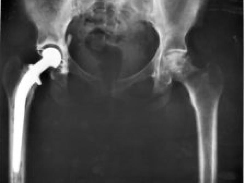
This research is carried out in the framework of MATHEON supported by Einstein Foundation Berlin. This project aims at a software environment supporting computer-assisted planning for total hip joint replacement by suggesting implant positions optimized for longevity of bone implants. The aim is to pre-operatively assess stress distribution in bone and to determine an optimal implant position with respect to natural function and stress distribution to prevent loosening, early migration, stress shielding, undesired bone remodeling, and fracture. Increasing the longevity of implants will help to enhance quality of life and reduce the cost of health care in aging societies. Focus of the research is the development of efficient optimization algorithms by adaptive quadrature of the high-dimensional space of daily motions and appropriate choice of tolerances for the underlying dynamic contact solver.
Introduction
Though we have an increased need of durable implants due to an aging society, the current implementation process still allows for improvement. Up-to-date software tools in computer-assisted hip implant surgery, e.g., still use 2D images of the patients hip geometry or have only begun to use 3D models. Loads which the implant has to endure on a daily basis are not considered at all and the joint socket is put in using the surgeons experience.
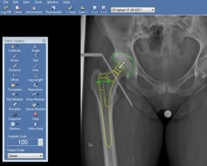
Figure: Current planning realized with 2D tools based on visual judgment and experience (e.g. Sectra PACS from Sectra)
The aim of this project is to optimize the hip implant position using a 3D, patient specific hip joint model. The natural range of motion is to be retained and stress induced by daily motions in a healthy hip joint is to be matched such that bone remodeling, dislocation, inflammation and pain is reduced or even prevented.
The numerical solution of this optimization problem is expensive. This is why methods have to be developed, that allow for a fast (or at least practical) computation of an optimal hip implant position. These methods need to take for example an adaptive approach on the load domain, that describes the daily motions. The error tolerance also needs to change adaptively, the optimization can be done with a multilevel approach and necessary refinement is to follow a goal-oriented error estimation scheme rather than a general error estimation scheme or, even worse, uniform refinement.
Underlying model
The bone is modeled as a linear hyperelastic, isotropic material. The included strain tensor (Cauchy-Green deformation tensor) can contain geometric non-linearity, but for the testing model the tensor is linearized. Arising ligaments and force densities acting on the joint through the ligament attaching points is put in by measuring the geometric (Euklidian) distance.
The FEM discretization and assembly of the according matrices is done using the Kaskade 7.3. The code is coupled with the FuFEM code from the Freie Universität Berlin in cooperation with the associated project ECMath CH1 – Reduced basis methods in orthopedic hip surgery planning. The FuFEM code contains the contact solver, that is described in this publication.
In order to have a computational inexpensive, but structurally realistic test setup for method development, simple 2D situations have been considered.
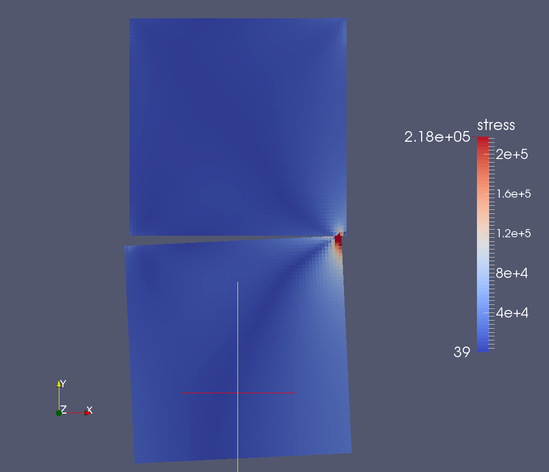
Figure: First contact computation on a simple two object geometry of two squares; the area of contact shows higher stresses; two ligaments are also modeled connecting the four proximate corners in an x pattern
The first computation has been conducted on a geometry of two squares. The more complicated geometry of a hip joint was acquired from ZIBAmira. For both geometries the Triangle code from Shewchuk was used, to get a first discretization.
The time varying force acting on the bottom boundary of the lower object is incorporated using a quasi-static approach.
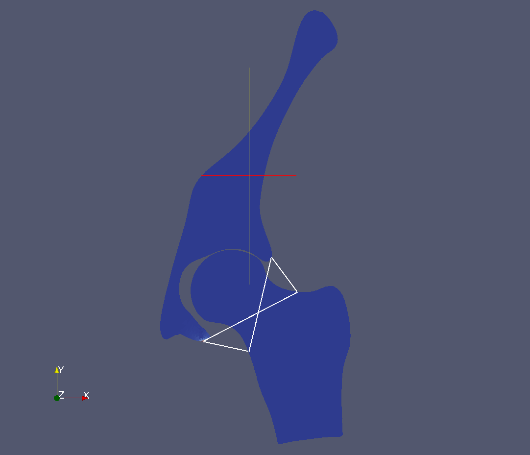
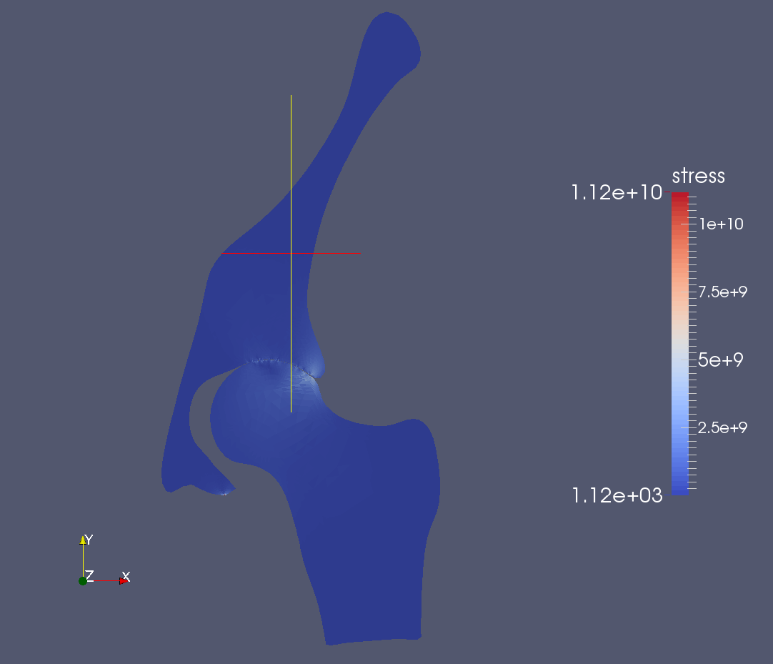
Figure: The hip joint is modeled with four ligaments (left) and with quasi-static contact (right)
Features like cartilage, muscles, soft tissues, a non-linearized deformation tensor, 3D geometry, Cosserat rods for the ligaments and others are possible (and eventually necessary), and will be included later.
Adaptive Optimization Challenges
The first challenge is the definition of an objective function. We consider objectives of the form:
\[J(p) = \int\limits_{m\in\mathcal{L}} \text{w}(m) \int\limits_{x\in\Omega} j(\sigma_{h}(p,m))\ \text{d}x\ \text{d}m\]
The basic idea is to optimize the implant's position p by computing the stresses sigmah – subscript h symbolizing the discretization of the geometry – induced through loads integrated over space. The function j penalizes high local stresses, yielding certain loads unfeasible that threaten to damage the bone, the implant's fixed position or are baneful in another way. The letter m stands for one motion from the parameter domain L where the loads are parametrized with angle, longitudinal and tangential forces, while the function w projects the load m to it's probability (walking and sitting loads being more frequent than stumbling or skiing loads).
This setup doesn't include retention of the natural range of motion yet which needs to be taken care of as well. Also the probability distribution of different loads and the penalization function j have to be designed.
Given the objective function, it is not clear whether it is continuous. This has to be studied and the (generalized) gradient will be derived, accordingly.
Afterwards methods can be developed, that ensure a fast and effective computation of an optimal position. In order to deal with the complexity of the parameter domain L, adaptivity in the choice of motion parameters is to be implemented. The selection of the motions happens according to the given probability distribution.
To even out numerical errors, this method will be combined with multilevel optimization. This combination will further be coupled with trust-region or line-search as well as goal-oriented error estimation methods.
On occurring position changes of the implant, forthcoming discretization errors will be analyzed and damped, such that they don't have a detrimental influence on finding an optimal implant position.
Dealing with errors will also take place in the method-development of adaptivity for the choice of error tolerance. Here we will start with a relatively coarse tolerance, which evolves fluently due to the optimization process, i.e. becoming increasingly fine according to the convergence and coarsening again on implant position changes, when the given differential equation has to be solved again for the chosen motions.
Which leads to the last part of the development. One has to look at the solution and decide what quantities will be stored for later use and comparison. The storage of the full spatio-temporal solution is infeasible, since that will exceed the available standard memory after a short time.
