Discrete-Continuous Free Flight Planning
The current system of routing flights on predefined airway networks does not harvest the benefits of exploiting tailwinds in an optimal way. Dropping the restriction to airways allows fuel to be saved and reduces CO2 emissions – an important driver in view of growing numbers of air traffic.
Established graph-based routing algorithms face considerable computational challenges in this setting. At ZIB, we develop and analyze hybrid approaches combining discrete optimization algorithms with optimal control methods in order to compute globally optimal free-flight trajectories to high accuracy in an efficient way.
The Future Sky
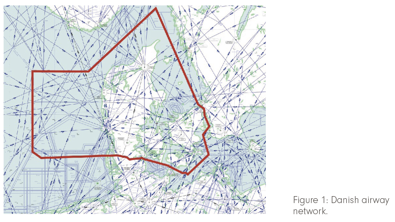
At the dawn of aviation, the sky was free, but navigation a problem. Apart from using a compass, the sun, moon, and stars, only landmarks and various sorts of beacons, vision and later radio provided orientation. Routes were set up between them, soon stacked into vertical flight levels, and monitored by air traffic control. In this way, today’s airway network evolved – a virtual 3D graph of 100,000 “waypoints” and 600,000–700,000 “segments” on each of 20+ flight levels, on which all air traffic takes place (see Figure 1 for an example). A notable exception was the oceans, where free flight was always possible, and very well exploited to cut short or to take advantage of favorable wind conditions.
At a long-term exponential growth of 4.4% per year, congestion of the airway network was unavoidable, and started to become more and more of a problem for at least a decade. On the other hand, aircraft navigation equipment became more and more sophisticated, reducing the need for centralized guidance. [Oxley, Jain 2015] (FN: Oxley, D., & Jain, C. / 2015. Chapter 1.4 Global Air Passenger Market: Riding OutPeriods of Turbulence, Travel and Tourism Competitiveness Report 2015. International Air Transport Association. World Economic Forum.)
Can one simply abandon the airway network to fly free like a bird, with a tailwind propelling you forward? This would eliminate congestion and detours, and save time, fuel, and emissions – a five-fold-win situation. It therefore doesn’t come as a surprise that the EU’s Single European Sky program has exactly this vision, and there are similar initiatives all over the world.
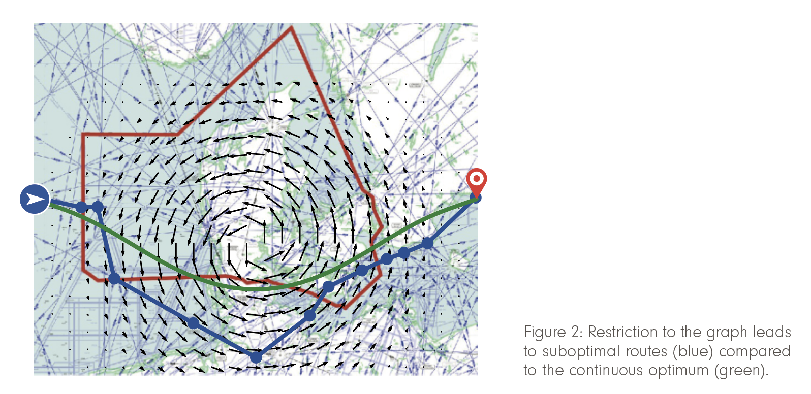
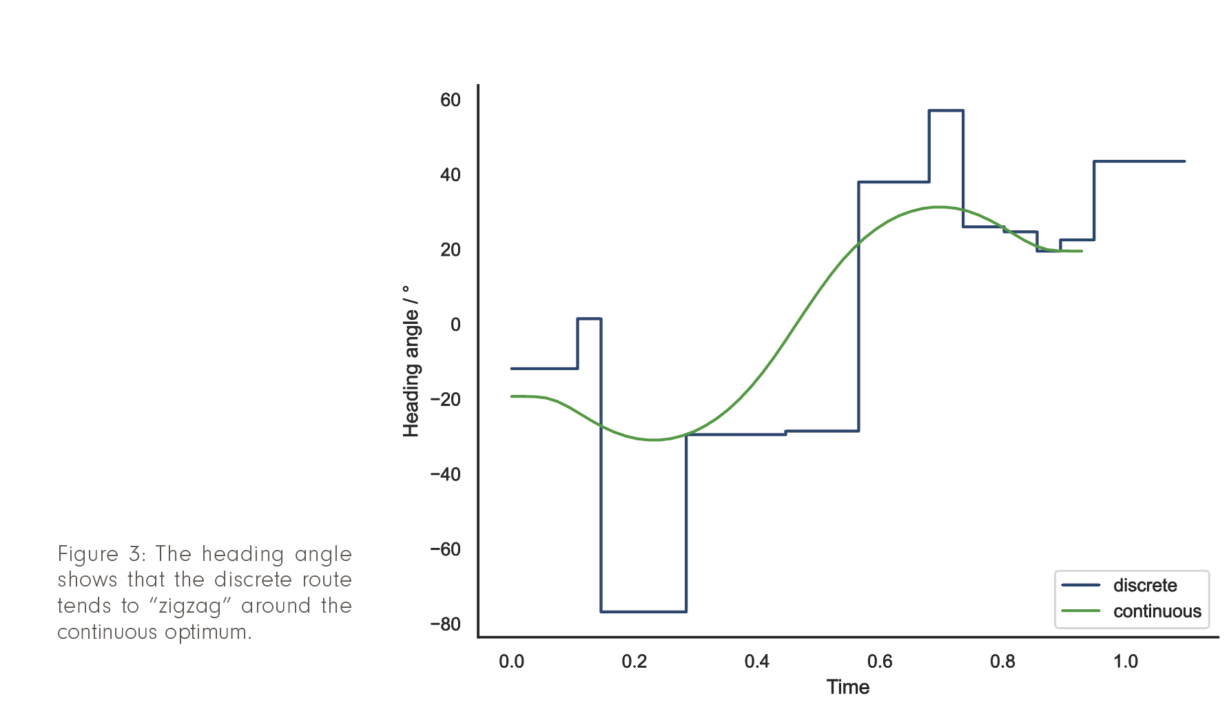
How much can one gain? Practical experience, recent studies [Wells et al. 2021], and our own numerical examples indicate potential savings in fuel and CO2 emission of about 2%, and up to 10% in extreme cases. As an example, consider Figure 2: the optimal free-flight route (in green) is not only faster, but also smoother in operation, as the comparison of the heading angles of both trajectories in Figure 3 shows.
To harvest these benefits, flight-planning tools are needed that can find the quickest, most fuel efficient, etc. free-flight route taking into account the weather conditions – and a number of other side constraints such as traffic rules – in reasonable time.
Discrete Flight Planning
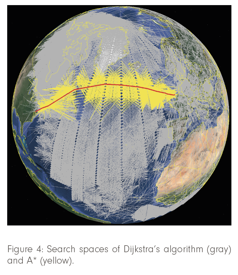
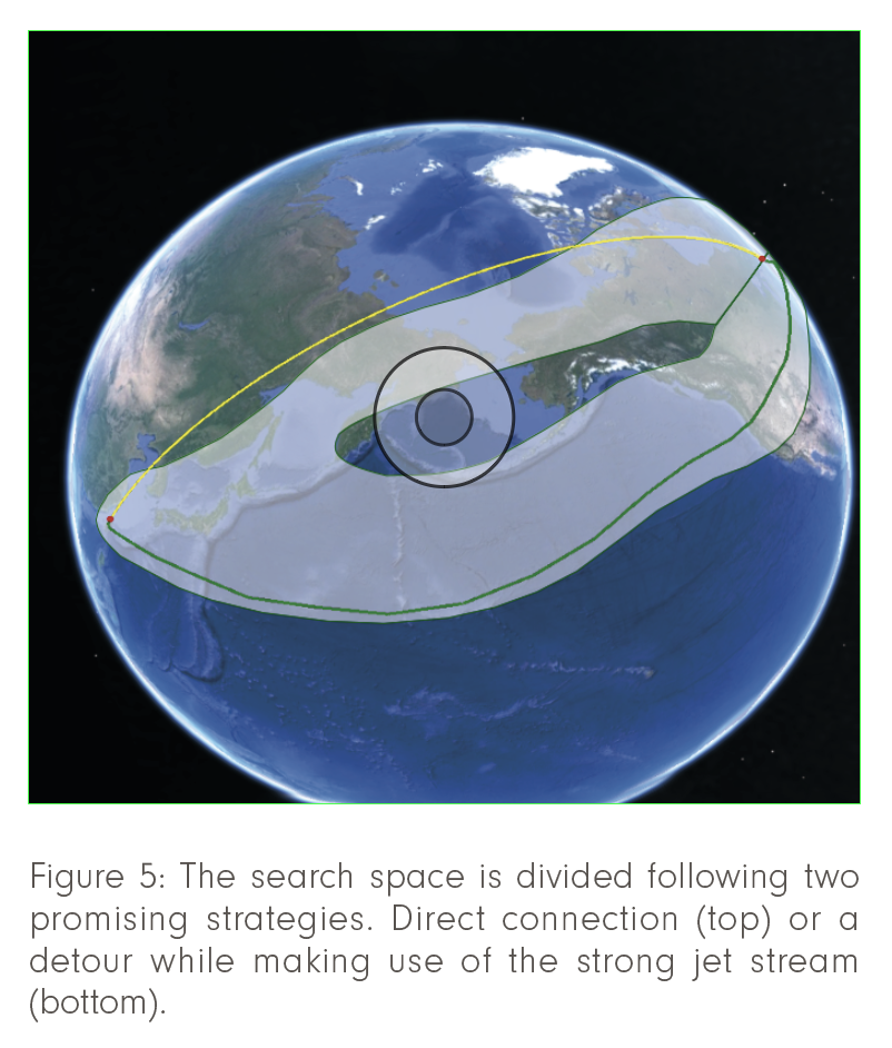
The current state of the art in flight planning is marked by discrete dynamic programming algorithms that are based on superfast shortest-path algorithms. These methods exploit the characteristics of the problem to derive powerful lower bounds that effectively prune the search space, such that globally optimal solutions can be computed to any desired degree of accuracy, with respect to several objectives, and subject to complex side constraints, including route availability, terrain clearance, alternate airport rules, etc. For example, bounds from so-called super-optimal winds, developed at ZIB in collaboration with Lufthansa Systems [Blanco et al., 2016] can be used to significantly tighten traditional A* bounds, which in turn already do much better than a pure Dijkstra approach, as illustrated in Figure 4. A striking example that stresses the importance of the wind is shown in Figure 5. The search space is subdivided into two routes, a northern direct route, and a longer southern corridor, which can take advantage of strong jet-stream winds, and, despite a detour of 1,250 km, turns out to save 45 minutes of flight time, 5.5 tons of fuel, 18.8 tons of CO2 and $1,100 of overflight fees.
For some time now, gradually expanding free-flight opportunities have been successfully approximated by graph densification (see Figure 6). However, this approach does not scale well, such that, at some point, the problem becomes intractable.
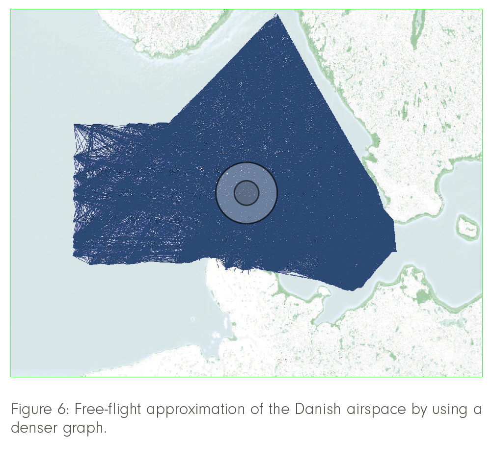
Indeed, the run time of discrete shortest-path algorithms depends on the density of the underlying network. On sparse graphs, shortest paths can be computed extremely fast by one of several domain-specific superfast algorithms. These all have a worst-case time complexity of O(|E| + |V| log|V|), where |E| and |V| are the number of edges and vertices, respectively. The airway network, like a planar graph, even has a favorably low number of edges: |E|=O(|V|), such that the overall runtime becomes a mere O(|V| log|V|), even without preprocessing. Naive free-flight networks, however, have a considerably larger number of vertices and |E|=O(|V|2) edges (see again Figure 6). This is an enormous difference, which at some point turns the computation of globally optimal shortest paths at high resolution and accuracy into an impossibility.
Continuous-Flight Planning
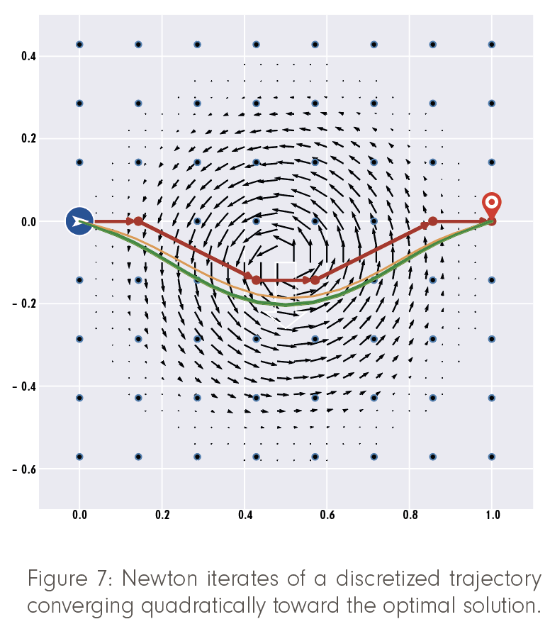
Continuous methods of optimal control, which have been studied for a century, are an algorithmic alternative. Instead of covering the airspace by a graph, they only discretize the trajectory itself, exploiting necessary optimality conditions to move the waypoints continuously in space (see Figure 7). Established methods based on Pontryagin’s maximum principle or direct collocation approximate the trajectories by higher-order polynomials, and thus translate the optimality conditions into large, sparse, and structured equation systems to be solved by Newton’s method. This allows much coarser discretizations to achieve the same accuracy as graph-based approaches, and, combined with fast quadratic convergence, highly accurate free-flight trajectories to be computed in a much shorter time frame.
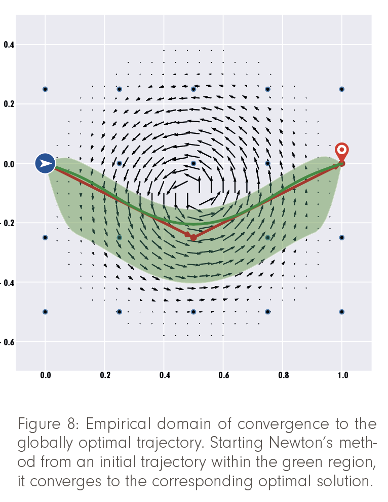
The downside of that approach is that these methods only converge to some nearby local optimum, if at all, and thus provide no guarantee of global optimality (see Figure 8). Thus, in itself, optimal control approaches are insufficient for free-flight planning.
The downside of that approach is that these methods only converge to some nearby local optimum, if at all, and thus provide no guarantee of global optimality (see Figure 8). Thus, in itself, optimal control approaches are insufficient for free-flight planning.
Can discrete and continuous methods be merged into an approach that combines their strengths and eliminates their weaknesses, resulting in a method that provides, at the same time, global optimality and rapid convergence to an optimal free-flight trajectory at any desired accuracy? Exactly this is the aim of a new method that is currently developed at ZIB: we recently proposed a novel hybrid algorithm called DisCOptER [Borndörfer/Danecker/Weiser2021].
A Hybrid Algorithm
While discrete, graph-based approaches efficiently approximate global optima at low to medium accuracy, continuous optimal control methods excel at fast local convergence to high accuracy. The hybrid DisCOptER method exploits these properties in a two-stage approach. In a nutshell, it starts an optimal control algorithm from a suitable path provided by a discrete dynamic programming method.
First, an artificial, fully connected graph is created (cf. Figure 10, blue dots) that contains origin and destination vertices. Then, a shortest path on this graph is calculated (red path).
Finally, this shortest path is used as an initial guess for the following refinement stage of the algorithm. Here, an optimal control approach involving some variant of Newton’s method is used to calculate a highly accurate solution (green trajectory). Provided that the first guess is within the radius of convergence of the actual continuous optimum (green area), Newton’s method converges extremely fast.
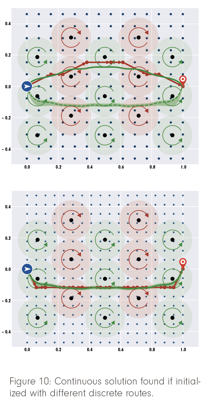
For the second stage to converge reliably to the global optimum in the vicinity of the path provided by the first stage, this path must be sufficiently close to the global optimum, more precisely, within the domain of convergence of Newton’s method. This can be ensured by making the first-stage graph sufficiently dense. The required graph resolution depends only on external factors like the wind conditions, but not on the desired accuracy, which only affects the trajectory discretization in the second stage.
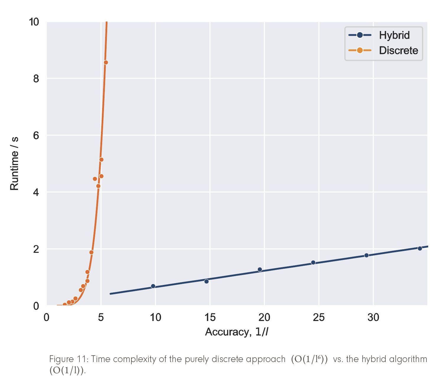
It turns out that in practically relevant examples, the required graph density is rather low (again, see Figure 10). Consequently, the discrete shortest path can be found quickly, the problematic asymptotic runtime behavior of the discrete graph search is circumvented, and the overall time complexity is governed by the asymptotically efficient optimal control stage (cf. Figure 11, 1/l is a measure for the solution accuracy). But can we decide within the algorithm how dense the graph needs to be in a concrete case?
Error Estimates for Discrete Paths
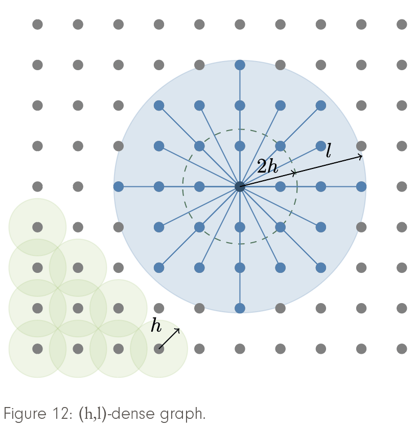
For free-flight trajectory planning, the graph used either stand-alone for path planning or as the first stage in a hybrid algorithm needs to be sufficiently fine for the discrete optimal path to be accurate enough or to lie within the convergence domain of Newton’s method, respectively. To ensure this, a priori error estimates for optimal flight paths in locally densely connected graphs have been derived [Borndörfer/Danecker/Weiser2021-b]. (h,l)-dense graphs are those where the h-balls around vertices cover the plane, and all vertices with a distance of l+2h at most are connected by an edge (see Figure 12).
Following the standard paradigm of a priori error estimates for finite element discretizations [Deuflhard/Weiser, 2020], the distance of an optimal continuous path to its interpolate in the graph is bounded, in terms of the flight duration, by bounding the second derivative of the objective with respect to path deviations. The structure of (h,l)-dense graphs guarantees the existence of a reasonable interpolant. Since the optimal discrete path in the graph is not worse than the considered interpolant, this provides an error bound for the discrete solution in terms of vertex density h, local connectivity length l, and magnitudes of wind speed and its spatial derivatives.
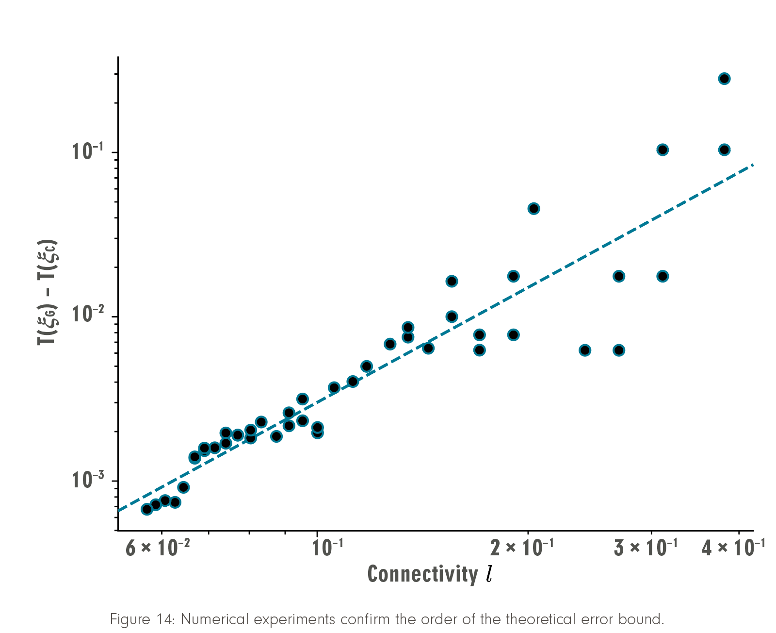
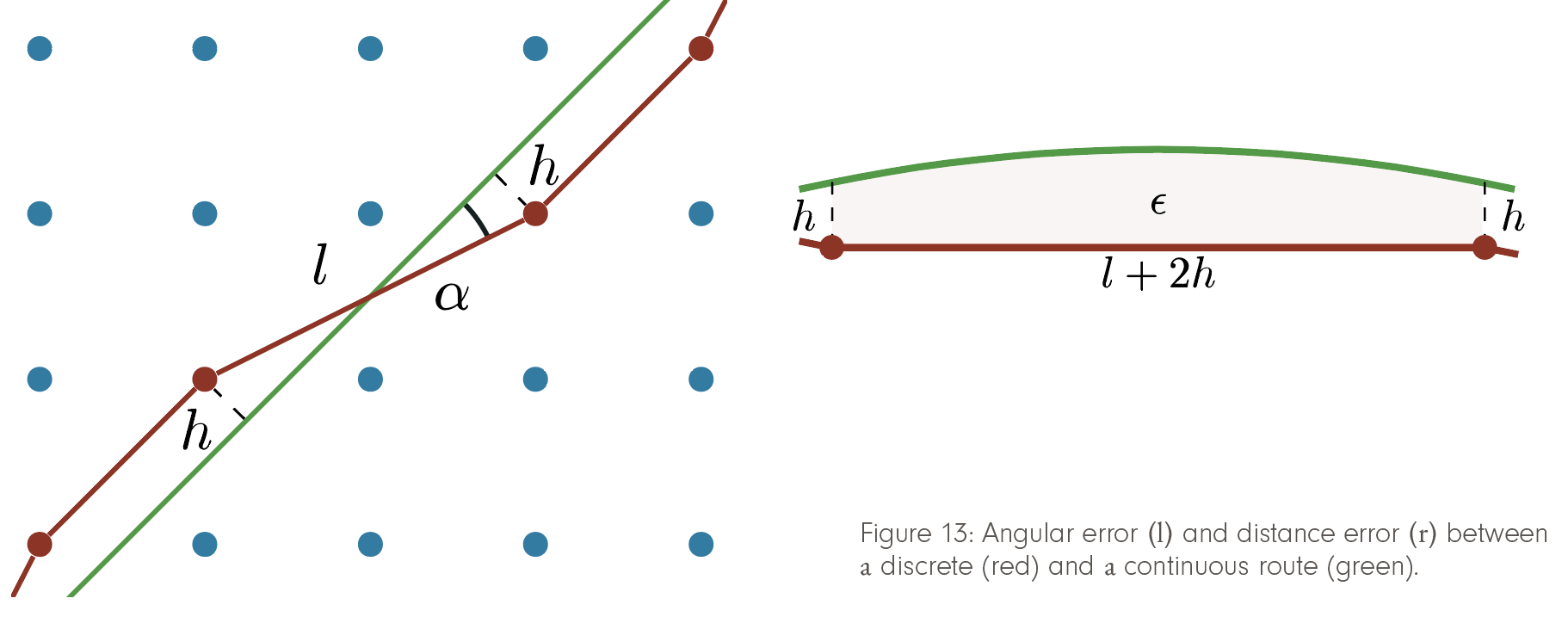
The excess in flight duration is due to spatial displacement of the trajectory on one hand, and zigzagging due to limited angular resolution on the other hand. The latter is bounded by l/h, whereas the former is controlled by h (see Figure 13). Based on this distinction, the error estimate allows the selection of a theoretically optimal relation of vertex density h and connectivity radius l, which turns out to be h = O(l2). The resulting error bound guarantees a convergence of optimal discrete paths toward the continuous optimum in terms of flight duration at a rate of O(l2).
As usual, the a priori error bounds are reliable but far from sharp. Nevertheless, they capture the numerically observed convergence order accurately (see Figure 14). This provides the basis on which efficient a posteriori error estimators can be designed, which can actually guide the graph refinement to the desired accuracy and allows implementing efficient and reliable hybrid algorithms.
DisCOptER is a first example of a new type of discrete-continuous algorithms that combine global optimality with fast local convergence. The underlying principle is not limited to shortest path problems, but is general enough to be applicable to many other problems of similar nature.