One aim of this project is to analyze a large set of medical image data with respect to the anatomy of the knee joint. The aim is to determine the variation in shape of the knee and knee joint space, respectively bone and cartilage, between distal femur and proximal tibia. Clusters of similar shapes have to be determined in order to design a limited set of knee spacers that fit a wide range of the osteoarthritic population.
Data selection
In order to detect different clusters of similar shapes at least 500 MRI datasets need to be processed. The datasets are taken from The Osteoarthritis Initiative (OAI) database. The OAI database contains about 5000 patients. Therefore, a selection has been made based on the Kellgren-Lawrence OA-Score which is available for almost all patients. The Kellgren-Lawrence score differentiates between five grades. For each of the five grades 138 female and 145 male patients have been randomly selected resulting in a preselection of 1415 right knee MRI datasets. In a first step 500 of these datasets are processed and analysed. As MRI protocol SAG_3D_DESS_WE (sagittal 3D dual-echo steady state with selective water excitation) is used for bone and cartilage segmentation.
Data processing
Bone and cartilage of distal femur and proximal tibia are segmented automatically using linear Statistical Shape Models (SSMs) [1]. Errors in the automatic segmentation are corrected manually. Additionally, for each knee landmarks of the insertion sites of anterior cruciate ligament (ACL) and posterior cruciate ligament (PCL) are placed by hand. A schematic overview is given in figure 1.
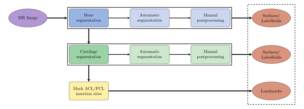
Fig. 1: Schematic overview of data processing
The following pictures illustrate the single steps of the pipeline.

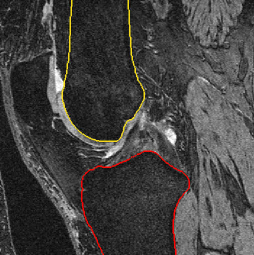
Fig. 2: Bone segmentation after automatic segmentation (left) and after manual postprocessing (right)
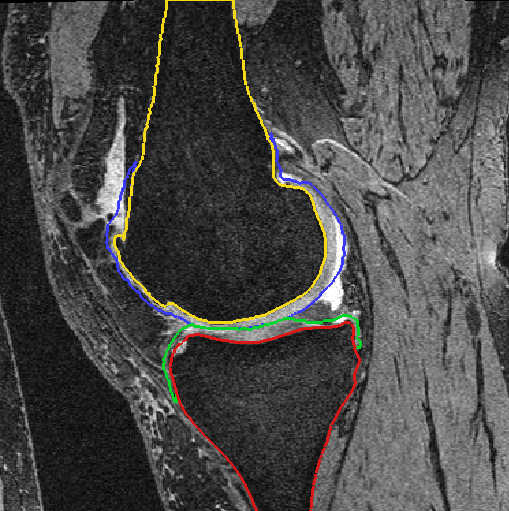
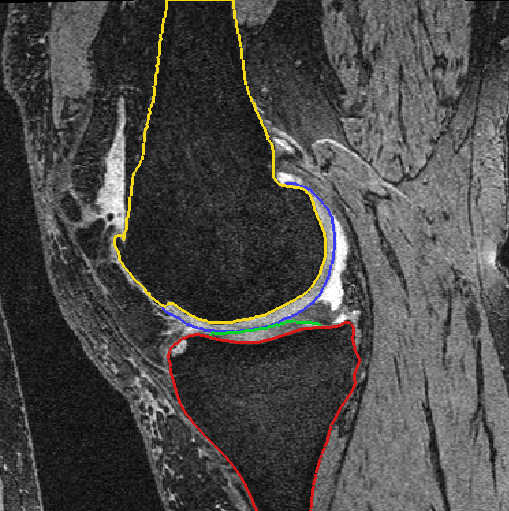
Fig. 3: Cartilage segmentation after automatic segmentation (left) and after manual postprocessing (right)
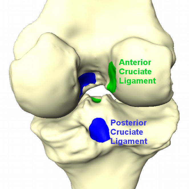
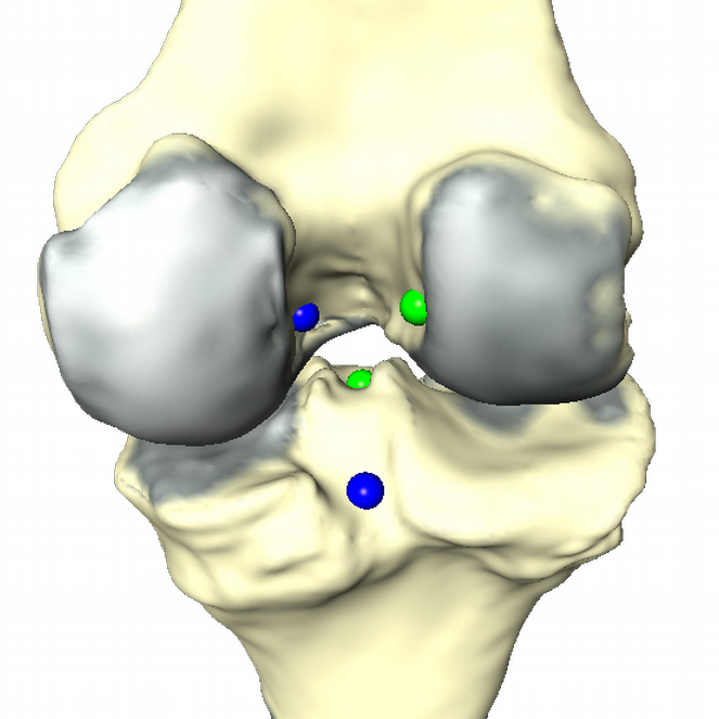
Fig. 4: Insertion sites of ACL and PCL (left). Result of data processing (right). Cartilage thickness is displayed in red. ACL and PCL insertion sites are replaced by a representative point.
Analysis
The aim is to find geometrical clusters in (very) high dimensional data. This fact complicates meaningful clustering. Therefore reduction of dimensionality/feature selection has to be done. Taking the geometries as triangular meshes there are different options how to proceed. One is the well known principal component analysis (PCA) on the vertex coordinates, that gives the SSMs, also known as Point Distribution Models (PDM). A more general approach is Principal Geodesic Analysis (PGA) [Ref Fletcher], which treats data as elements in a Riemannian manifold and carries out statistical operations therein or in the tangential space to a reference element respectively. This procedure has the advantage that it can be sensible to nonlinear shape changes depending on the chosen modeling space. It should be noted that PCA can be interpreted as special case of PGA, namely with the flat Euclidean space as underlaying manifold. We develop a method that employs the deformation gradient of a mesh modeled as element of a Lie group and thus delivering an even richer mathematical structure. It is called the Gradient Domain Model (GRM).
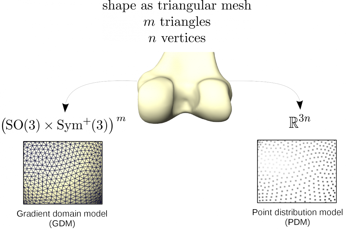
Fig. 5: Used properties of a mesh with respect to the chosen shape model.

Fig. 6: Principal Geodesic Analysis on a Lie group G schematically done on a sphere.
OA related changes of distal femur
The distal femur exibits clear pathological changes in case of a severe OA and is therefore an interesting structure to take into consideration for Clustering and Classification of OA.

Fig. 7: Healthy (left) and osteoarthritic (right) distal femur with delineated pathological changes in shape.
Classification and Clustering
To find clusters we apply our GDM on patients that are healthy (KL 0/1) and those that are severely deseased (KL 4). The resultant shape weights are used to train a Support Vector Machine in order to classify between this two groups.
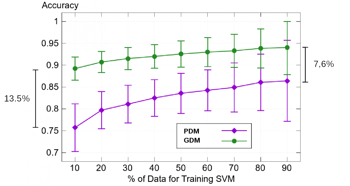
Fig. 8: Classification results for 58 severely deseased (KL4) and 58 (almost) healthy (KL0/1) femurs.
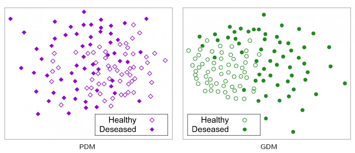
Fig. 9: Sammon Projection for 58 severely deseased (KL4) and 58 (almost) healthy (KL0/1) femurs.
References
[1] Seim, H., Kainmueller, D., Lamecker, H., Bindernagel, M., Malinowski, J., & Zachow, S. (2010). Model-based auto-segmentation of knee bones and cartilage in MRI data. Proc. MICCAI Workshop Medical Image Analysis for the Clinic - A Grand Challenge, 215-223.